Toast toolbox tutorial: Demonstrating non-uniqueness

This example demonstrates a non-uniqueness condition in DOT. Transillumination amplitude data from a steady-state measurement at a single wavelength are not sufficient for reconstructing both absorption and scattering parameter distributions.

In this example, this is demonstrated by generating data from a model with homogeneous absorption, while scattering consists of a homogeneous background with a circular inclusion of increased scattering.

Using these data, an absorption-only reconstruction is performed under the assumption that scattering is constant.

The reconstruction succeeds in finding an absorption distribution that generates data matching the scatter-perturbed target data.

The Matlab script for this example can be downloaded here.

Step 1: Create the target mesh

For this example, we create a 2D circular mesh with a circular inclusion. You can create this mesh yourself with gmsh (see Meshing tutorial 1 and Meshing tutorial 2 for details). The mesh should be circular with radius 25 and centre in the origin. It should contain a small off-centre inclusion, and separate surface definitions for the background and inclusion. Call the mesh circle_blob.msh so that the script will recognise it.

Alternatively, you can download a ready-made mesh here.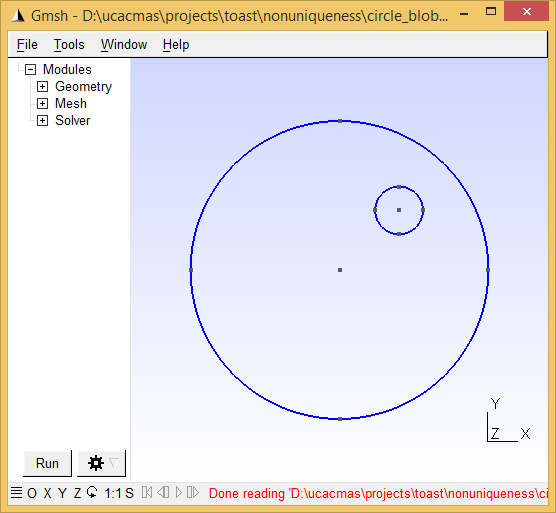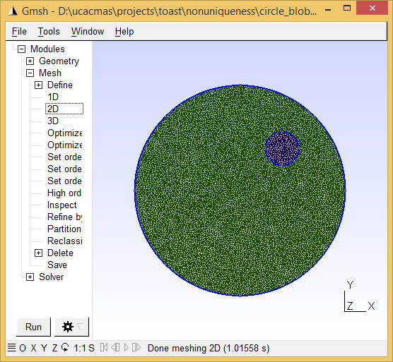

Step 2: Load the mesh

We start the script by loading the mesh and identifying the elements forming the inclusion:

mesh = toastMesh('circle_blob.msh','gmsh');
ne = mesh.ElementCount;
nv = mesh.NodeCount;
regidx = mesh.Region;
regno = unique(regidx);
blobel = find(regidx == regno(2)); % assuming that the second surface marks the inclusion

Step 3: Define source and measurement geometry

We define 32 source and detector locations along the mesh circumference, and use toastMesh methods Qvec and Mvec to extract the corresponding operators.

rad = 25; % mesh radius [mm]
nopt = 32;
for i=1:nopt
  phiq = (i-1)/32*2*pi;
  qpos(i,:) = rad*[cos(phiq), sin(phiq)];
  phim = (i-0.5)/32*2*pi;
  mpos(i,:) = rad*[cos(phim), sin(phim)];
end
mesh.SetQM(qpos,mpos);
qvec = real(mesh.Qvec('Neumann','Gaussian',2));
mvec = real(mesh.Mvec('Gaussian',2,refind));

Step 4: Define the target parameter distribution

We want a piecewise constant target parameter distribution, so the target parameters are assigned in an element basis:

refind = 1.4; % refractive index
c0 = 0.3; % speed of light in vacuum [mm/ps]
cm = c0/refind; % speed of light in the medium [mm/ps]
mua_bkg = 0.01; % background absorption [1/mm]
mus_bkg = 1; % background scattering [1/mm];
ref = ones(ne,1)*refind;
mua = ones(ne,1)*mua_bkg;
mus = ones(ne,1)*mus_bkg;
mus(blobel) = mus_bkg*2;

% Display the target distributions
figure('position',[0,0,640,420]);
subplot(2,3,1); mesh.Display(mua, 'range',[0.005,0.025]);
axis off; title('\mu_a target');
subplot(2,3,2); mesh.Display(mus, 'range',[0.8,2.2]);
axis off; title('\mu_s target');

Step 5: Generate target data

Use the FEM solver to generate surface CW amplitude data for the model defined above. Also solve the homogeneous problem to allow display of perturbation data:

% compute perturbed target model
smat = dotSysmat(mesh, mua, mus, ref, 'EL');
data = log(mvec' * (smat\qvec));

% for reference, also solve the homogeneous problem
mus = ones(ne,1)*mus_bkg;
smat = dotSysmat(mesh, mua, mus, ref, 'EL');
data_homog = log(mvec' * (smat\qvec));

% display sinogram of target data perturbations due to inclusion
subplot(2,3,3);
imagesc(data-data_homog, [-0.26,0.015]); axis equal tight; colorbar
title('target data');

Note the 'EL' flag in the system matrix computation. This signals to Toast that the parameter vectors are supplied on an element-wise basis (default is node basis).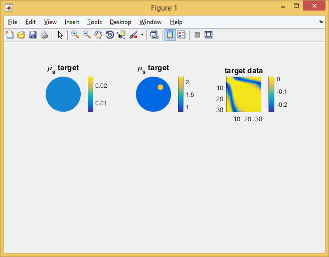

Step 6: Setting up the inverse solver

For the reconstruction, we start from the correct background parameters. However, the reconstruction will (wrongly) assume that the scattering distribution is homogeneous, and only update the absorption distribution.

To initialise the inverse solver, we reset the parameters to their background values, and compute the corresponding FEM solution. Note that for the inverse problem, we assume piecewise linear parameter distributions, and therefore define the parameters on a nodal basis.

mua = ones(nv,1)*mua_bkg;
mus = ones(nv,1)*mus_bkg;
ref = ones(nv,1)*refind;
smat = dotSysmat(mesh, mua, mus, ref);
proj = reshape(log(mvec' * (smat\qvec)), [], 1);
sd = ones(size(proj));
data = reshape(data, [], 1);
subplot(2,3,4); mesh.Display(mua, 'range',[0.005,0.025]); axis off; title('\mu_a recon');
subplot(2,3,5); mesh.Display(mus, 'range',[0.8,2.2]); axis off; title('\mu_s recon');
subplot(2,3,6); imagesc(reshape(proj,nopt,nopt)-data_homog, [-0.26,0.015]); axis equal tight; colorbar
title('recon data');

Next, we set up an inverse solver basis as a regular 32x32 grid, and map the intial estimate of the solution vector (the log of the absorption distribution) into that basis.

grd = [32,32];
basis = toastBasis(mesh, grd);

bmua = basis.Map('M->B', mua);
bcmua = bmua*cm;
scmua = basis.Map('B->S', bcmua);
x = scmua;
logx = log(x);
slen = length(x);

We set up a regularizer instance and compute the initial value of the objective function:

regul = toastRegul('TV', basis, logx, 1e-4, 'Beta', 0.01);

err0 = toastObjective(proj, data, sd, regul, logx);
err = err0;
errp = inf;
itr = 1;
step = 1.0;
fprintf('Iteration %d, objective %f\n', 0, err);

Step 7: The inverse solver loop

Finally, we add the loop for the iterative minimisation of the objective function. Note that this uses a local callback function for the evaluation of the line search. Therefore, Matlab requires that the main body of the code is wrapped into a function as well:

function nonuniqueness

% -------------------------
% code so far
% -------------------------

% inverse solver loop
itrmax = 100; % CG iteration limit
tolCG = 1e-6; % convergence criterion
while (itr <= itrmax) && (err > tolCG*err0) && (errp-err > tolCG)

  errp = err;
  r = -toastGradient(mesh, basis, qvec, mvec, mua, mus, ref, 0, ...
    data, sd, 'method', 'cg', 'tolerance', 1e-12);
  r = r(1:slen); % drop mus gradient
  r = r .* x; % parameter scaling
  r = r - regul.Gradient(logx);

  % CG search direction update
  if itr > 1
    delta_old = delta_new;
    delta_mid = r' * s;
  end
  s = r;
  if itr == 1
    d = s;
    delta_new = r' * d;
  else
    delta_new = r' * s;
    beta = (delta_new - delta_mid) / delta_old;
    if mod(itr, 20) == 0 || beta <= 0
      d = s;
    else
      d = s + d*beta;
    end
  end
  % Line search along update direction
  step = toastLineSearch(logx, d, step, err, @objective);
  logx = logx + d*step; % update solution estimate
  mua = basis.Map('S->M',exp(logx)/cm);
  subplot(2,3,4); mesh.Display(mua, 'range',[0.005,0.025]);
  axis off; title('\mu_a recon');

  proj = reshape(log(mvec' * (dotSysmat(mesh, mua, mus, ref)\qvec)), [], 1);
  subplot(2,3,6); imagesc(reshape(proj,nopt,nopt)-data_homog, [-0.26,0.015]);
  axis equal tight; colorbar
  title('recon data');
  err = toastObjective(proj, data, sd, regul, logx);
  fprintf('Iteration %d, objective %f\n', itr, err);
  itr = itr+1;
  drawnow
end

  function p = objective(logx)

    mua_ = basis.Map('S->M',exp(logx))/cm;
    proj_ = reshape(log(mvec' * (dotSysmat(mesh, mua_, mus, ref)\qvec)), [], 1);
    p = toastObjective(proj_, data, sd, regul, logx);

  end

end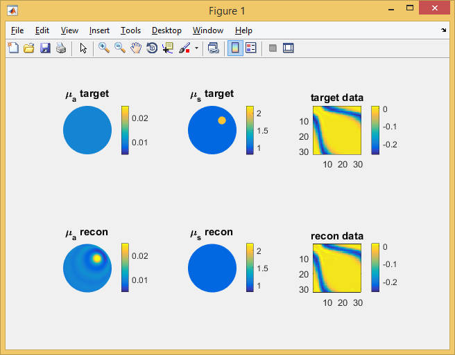

The image above shows the result of the absorption reconstruction after 100 CG steps. It produces an absorption feature in approximately the position of the actual scattering object, and oscillatory rings around it. The boundary data generated by this absorption distribution match those of the target scattering distribution (right column), with an objective function of 0.0067 from the initial value of 8.26 of the homogeneous starting distribution.

Further experiments

As a further exercise, modify the reconstruction script so that it uses frequency domain data (log amplitude and phase) for the absorption reconstruction. Does the inverse solver still find a solution that agrees with the target data?
Try to reconstruct both absorption and scattering from amplitude-only data. What happens?