| Image Reconstruction in Optical Tomography |
|
|
Introduction Download Documentation Support |
Toast python module tutorial: Building a DOT forward solverThis example shows how to write a simple DOT steady-state forward solver in python using the Toast module. To run this code yourself, you need python with the numpy, scipy and matplotlib modules, as well as the Toast python module. To save you typing, the full python script for this example can be downloaded here. Step 1: PreliminariesWe need to import a few standard modules:
import os
and set up the toast module:
import sys import numpy as np from numpy import matrix from scipy import sparse from scipy.sparse import linalg from numpy.random import rand import matplotlib.pyplot as plt
execfile(os.getenv("TOASTDIR") + "/ptoast_install.py")
from toast import mesh
Note that the ptoast_install script simply sets up the search paths for the local installation of the toast python module. If you installed the toast module in python's default module location, you can skip this line.
Step 2: Load a meshThe forward solver uses the finite element method to solve the diffusion equation in a domain. An unstructured mesh is required to define the domain and distribution of parameters. For this example, we load a simple 2-D circular mesh stored in a file:
meshdir = os.path.expandvars("$TOASTDIR/test/2D/meshes/")
meshfile = meshdir + "circle25_32.msh" qmfile = meshdir + "circle25_32x32.qm" hmesh = mesh.Read(meshfile) The function should respond with the message
Mesh: 3511 nodes, 6840 elements, dimension 2
189 boundary nodes The geometrical mesh data (node positions and element connectivity) can be extracted from the mesh handle with:
nlist,elist,eltp = mesh.Data (hmesh)
nlen = nlist.shape[0] where nlist is an array of node coordinates, elist is the element connectivity list, and eltp is a list with element type identifiers. nlen is the number of nodes, used later in the script. Step 3: The optical coefficientsThe forward solver requires the distribution of absorption and scattering coefficient, as well as the refractive index. The mesh defines a basis u(r) with which functions f(r) defined in the domain can be approximated with a finite dimensional array of coefficients: 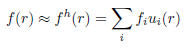
In this example, we assume a piecewise linear basis, where coefficients fi are defined on the vertices of each mesh element. (Toast also allows to define a piecewise constant basis, as well has higher-order polynomial bases. We'll come to those later.) Toast constructs the basis ui(r) automatically. All we have to provide are the index arrays for absorption μa, scattering μs and refractive index n:
mua = np.ones ((1,nlen)) * 0.025
mus = np.ones ((1,nlen)) * 2.0 ref = np.ones ((1,nlen)) * 1.4 mua, mus and ref now homogeneous parameter distributions. We will look at creating inhomogeneous distributions later. Source and detector locationsWe need to define at least one source distribution and one detector profile for the forward solver. For practical applications, multiple source and detector locations are usually employed. For this example, we read a list of source and detector locations predefined in a file, and associate it with the mesh:
mesh.ReadQM(hmesh,qmfile)
From the source and detector locations, you create the source and boundary projection vectors using the mesh.Qvec and mesh.Mvec functions:
qvec = mesh.Qvec (hmesh)
mvec = mesh.Mvec (hmesh) Running the forward solverWe now have everything in place to set up and run the forward solver to simulate the measuremenets for our problem. The FEM formulation leads to a linear system of the form 
where K is a system matrix depending on the parameters x (absorption, scattering, refractive index), Q is a matrix of column vectors, where each column consists of one source distribution, M is a matrix of column vectors for the detector response distributions, %Phi; is the matrix of photon density distributions for each source, and Y contains the measurements for each source and detector combination. With the Toast module, this system is represented by the following code
smat = mesh.Sysmat (hmesh, mua, mus, ref, 0)
nq = qvec.shape[1] phi = np.zeros((nlen,nq),dtype=np.cdouble) for q in range(nq): qq = qvec[:,q].todense() res = linalg.bicgstab(smat,qq,tol=1e-12) phi[:,q] = res[0] where mesh.Sysmat builds system matrix K from the mesh geometry and parameter coefficients (the '0' at the end refers to the modulation frequency, which is zero for a steady-state problem). The sparse linear system is solved for Φ using the iterative BiCGSTAB solver provided with scipy. Other solvers such as GMRES are also available.
We now need to map the fields to boundary measurements by projecting onto the measurement profiles, and convert to logarithmic data:
y = mvec * phi
logy = np.log(y) You can display the measurements as a sinogram, using matplotlib plotting functions:
plt.figure(1)
im = plt.imshow(logy,interpolation='none') plt.title('log amplitude') plt.xlabel('detector index') plt.ylabel('source index') plt.colorbar() plt.draw() 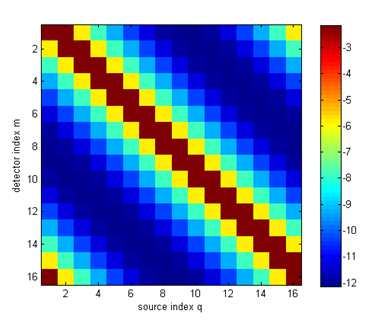
|