Tutorial: Connectivity-based segmentation of the corpus callosum

This tutorial uses Camino to perform a connectivity-based segmentation of the corpus callosum. The methods are explained in more detail in [1]. We use a single brain from the data set of [1], which is also used in the tractography tutorial. Unlike [1], we fit a single diffusion tensor to each voxel in the brain using the standard linear reconstruction.

In addition to doing the segmentation, the tutorial shows some other options to process tractography data.

Reconstructing the data

We begin with the data in voxel order in the file scans/brain.Bfloat. The reconstruction is the same as in the tractography tutorial, so we'll just recap briefly here.

Step 1 is to get the tensors:

$ dtfit scans/brain.Bfloat scans/tensorPoints.scheme > scans/brainDT.Bdouble

Step 2 is to define the PICo [2] PDFs. First, we define the lookup table that maps tensor shape to the estimated uncertainty for that tensor, given the imaging scheme. This step only needs to be done once for all subjects acquired using the same scheme.

$ dtlutgen -schemefile scans/tensorPoints.scheme -snr 16.0 -inversion 1 > scans/picoTable.dat

Then we get the PDFs for the particular data set. This step needs to be done for each subject, but is faster than computing the lookup table.

$ picopdfs -inputmodel dt -luts scans/picoTable.dat > scans/brainDT_pico.Bdouble

Now we are ready to do some tracking.

The grey matter atlas

The atlas is defined in [3] and contains labels for 52 regions of the brain. The labels are defined in a T1-weighted template image from the Brainweb project. The labels were warped into the space of the subject's diffusion image by calculating a warp from the template to the subject T1, and then from the subject T1 to the diffusion image. We define a mask of the atlas, which we will use to restrict the analysis to pathways that enter the labelled regions. This is easily done in Matlab:

>> fid = fopen('/scans/atlas_subject.img', 'r');
>> atlas = fread(fid, 'int');
>> fclose(fid);
>> mask = atlas ./ atlas;
>> fid = fopen('/scans/atlas_mask.img', 'w', 'b');
>> fwrite(fid, mask, 'int16');
>> fclose(fid);

A header is required for the mask image.

$ analyzeheader -voxeldims 1.7 1.7 2.3 -datadims 128 128 60 -datatype short > scans/atlas_mask.hdr
See also the Camino program for another way to create the mask.

Tracking from the corpus callosum

Before running a lengthy PICo process, we'll track a few streamlines to make sure that everything is set up correctly. The ROI in the corpus callosum is defined by hand in SNAP.

$ track -inputmodel pico -inputfile scans/brainDT_pico.Bdouble -seedfile scans/cc_b0.hdr -iterations 10 | procstreamlines -waypointfile scans/atlas_mask.hdr -exclusionfile scans/atlas_mask.hdr -truncateinexclusion > picoTracts.Bfloat $ vtkstreamlines -targetfile scans/atlas_subject.hdr -inputfile picoTracts.Bfloat > pico.vtk

The call to does a couple of things. First, we use the mask as a "waypoint" image. That is, any streamlines that do not enter the mask are discarded. Secondly, we use the mask as an "exclusion" image. By default, streamlines that enter an exclusion image are discarded, but the -truncateinexclusion option tells the program to cut the streamline when it enters the mask.

The command converts the streamlines into VTK polylines, which we can view in Paraview. The target file is passed to vtkstreamlines to tell it to colour each streamline by the target region to which it connects. The image below shows the streamlines and the outline of the atlas mask.

We can now do the PICo tracking for real, with 1000 iterations per voxel. We'll save the results to disk, so we can do different analyses without re-running the tractography. In order to save disk space, we save each streamline as a list of voxels in the diffusion image space, and use the gzip algorithm to compress the output.

$ track -inputmodel pico -inputfile scans/brainDT_pico.Bdouble -seedfile scans/cc_b0.hdr -iterations 1000 -outputtracts voxels -gzip > picoVoxels.Bshort.gz

Connection probabilities to the grey matter targets

Camino offers a number of options for dealing with probabilistic streamlines. The simplest thing is to make an image of the PICo from each seed point. This is an Analyze image where the intensity in each voxel is the fraction of streamlines from a particular seed point that intersect that voxel. To do this, we run

$ procstreamlines -inputfile picoVoxels.Bshort.gz -inputmodel voxels -outputcp -iterations 1000 -seedfile scans/cc_b0.hdr -outputroot scans/cc_cp_ -gzip

The output is one Analyze image per seed point. The output files are named cc_cp_1_*_1.[hdr, img.gz], where * is the seed point (1 through N for N seed points). The last index is the principal direction in the seed voxel. If there are multiple fiber orientations in a seed voxel, a separate image is generated by following each one.

Next, we get the fraction of probabilistic streamlines that connect to each target region by specifying the atlas as a target file. The output is an Analyze image for each seed, as before, except this time the intensity of each voxel in the target file is the PICo to that target, and the intensity of all other voxels is zero. This time, we also use the mask as a waypoint file, so streamlines that do not connect to any region of interest are discarded.

$ procstreamlines -inputfile picoVoxels.Bshort.gz -inputmodel voxels -outputcp -iterations 1000 -seedfile scans/cc_b0.hdr -targetfile scans/atlas_subject.hdr -waypointfile scans/atlas_mask.hdr -outputroot scans/cc_targetcp_ -gzip

Any connection probability image can be passed to to get the maximum, minimum, mean, or median value over all seed points in an ROI. We'll get the mean target connection probability over all seed points:

$ cpstats -operation mean -inputroot scans/cc_targetcp_1_ -targetindex 0 -outputfile scans/cc_meancp

The result is shown below.

The command converts the target connection probabilities to a text file. The command in this example is

$ targetprobs2txt -inputroot scans/cc_targetcp_ -seedfile scans/cc_b0.hdr -targetfile scans/atlas_subject.hdr > targetcp.txt

For each seed point, the output is x y z cp_1 cp_2 ... cp_T where each seed point is voxel [x, y, z] in the seed file, and there are T targets in the target file.

Connectivity segmentation of the corpus callosum

We perform the connectivity segmentation with the command

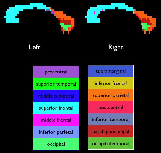
There are two differences to the earlier commands: we specify -outputcbs option, which tells the program to do the connectivity segmentation. Also, we specify that the partition should be bi-directional, ie the program should output a separate segmentation for the streamlines tracked in each direction from the seed point. The vector [1 0 0] is the normal to the plane that divides the streamlines at the seed point. In the case of the corpus callosum, the fibers run left-right at the mid-sagittal, so we compute a separate segmentation for left and right connections. The command above outputs four images: ${outputroot}labels_1_1_[0,1] and ${outputroot}labelcp_1_1_[0,1].

The numbering scheme for the output is as follows: ${outputroot}[labels, labelcp]_${seed ROI}_${principal direction}_[0,1]. We only have one seed ROI in this case, and there is only one principal direction (PD) in each voxel. The last value is 0 for the connections towards the vector we specified with -directional. In this case, the connections to the right side of the brain are in the images _0.[hdr,img].

In the "labels" image, each seed point is assigned the value of the target to which it has the highest connectivity (see image below). The "labelcp" image contains the PICo for the target with the highest connectivity: the value in each seed point is the fraction of the total streamlines (1000 in this case) that connect to the target region specified in the "labels" image. The "labelcp" image gives an indication of the confidence in the target labeling (higher is better). A more detailed analysis of the labeling is possible using the output from targetprobs2txt.

References

[1] Cook P A, Zhang H, Avants B, Yushkevich P, Alexander D C, Gee JC, Ciccarelli O, Thompson A J, An Automated Approach to Connectivity-based Partitioning of Brain Structures, LNCS 3749, p. 164-171, 2005

[2] Parker G J M, Haroon H A and Wheeler-Kingshott C A M, A Framework for a Streamline-Based Probabilistic Index of Connectivity (PICo) using a Structural Interpretation of MRI Diffusion Measurements, Journal of Magnetic Resonance Imaging 18:242-254, 2003

[3] Yushkevich P, Dubb A, Xie Z, Gur R, Rur R, Gee J, Regional Structural Characterization of the Brain of Schizophrenia Patients, Academic Radiology 12:1250-1261, 2005