Tutorial: Using Camino for Tractography
This tutorial uses Camino to perform tractography on diffusion tensor data. We will produce images using both streamline and probabilistic tractography using the PICo algorithm [1][2][3]. The Camino toolkit is designed to be modular, with different programs performing different tasks being linked together by "piping" the output of one program to the input of the next. In this way it is possible to construct highly flexible processing "pipelines" which take raw scanner data and output the processed results in the desired format. This case study assumes almost no knowledge of either the Camino toolkit or POSIX scripting.
Data pipelines are easily constructed using UNIX shell commands. The pipe operator "|" (this is a vertical line, sometimes printed with a gap in the middle. On UK keyboards this is shift-backslash) is used to make the output of one command as input to another. In this way it is possible connect sequential processing steps together without the need to generate intermediary data-files. This case study assumes that you are using some form of shell with pipes, these include most UNIX shells such as bash, csh, tcsh and ksh but not MS-DOS. The best way to use Camino in a windows environment is to install a UNIX emulator, such as Cygwin. While we will often pipe several commands together, it is often useful to save the output of Camino programs so that they may be re-used. For example, the command
cat scans/brainDT.Bdouble | dteig | pdview -datadims 128 128 60
is equivalent to
cat scans/brainDT.Bdouble | dteig > scans/eig.Bdouble; cat scans/eig.Bdouble | pdview -datadims 128 128 60
but the second version saves the tensor eigen system for later use.
The command syntax used in this case study assumes that data is contained in a directory called scans in present directory. The PICo stage of the case study also makes use of a subdirectory scans/pico/ for the intermediate images which are used to compile the final connection probability image.
The commands themselves are contained in the camino/bin directory. To let the shell you are using know to look for commands in this directory, type
set path = ( $PATH CAMINO_DIR/bin )
replacing CAMINO_DIR with the directory Camino is installed in. If you are using Camino frequently, it is a good idea to add this line to your .cshrc file, below any other set path ... statements. Alternatively, cd to camino/ and type bin/COMMAND instead of COMMAND in each of the example commands given in this case study.
At each stage of the process we give an indication of how long each step might take. These times are estimates based on the time taken to perform each step on a 3.2GHz P4 Linux PC.
Data
Tractography algorithms require directional data. This case study performs diffusion tensor tractography and hence as part of the analysis we will discuss how to fit diffusion tensors to scanner data using Camino.
The data used here was acquired using 66 acquisition directions, diffusion time Delta= 0.04s and Gradient strength G= 0.022Tm-2. Images were acquired over a whole brain with 128x128x60 voxels of dimension 1.7mm x 1.7mm x 2.3mm. It was kindly provided by Claudia Wheeler-Kingshott, Olga Ciccarelli and Alan Thompson, Department of Headache, Brain Injury and Neurorehabilitation, Institute of Neurology, UCL. The data is prepared in big-endian voxel order format, which is the format required by Camino. Data produced by scanners is frequently little-endian, image order or both. Camino contains modules for changing endian-ness of data and converting scanner-order data in voxel order. This is discussed in the Pig Brain tutorial. The pig brain tutorial also explains how to make a schemefile from a list of gradient directions. The data file name in this tutorial is brain.Bfloat where the extension .Bfloat indicates that the data in this file is in the form of big-endian floats (4 byte floating-point numbers).
Scheme File
The schemefile tells Camino about scan parameters and directions. There are several ways to describe the imaging scheme, the simplest and most commonly used is a list of gradient directions and associated b-values.
# Camino scheme file - X Y Z b for each measurement
VERSION: BVECTOR
0    0    0    0
1    0    0    1000
0    1    0    1000
0    0    1    1000
...
The gradient directions should be listed in order for each measurement. They should also be normalized to unit length (if they are not, they will be normalized at run time). The b-values determine the scale of your diffusion tensors - in the example above, we've used a b-value of 1000 s / mm^2, which is standard for DTI. If we want tensors in SI units (meters and seconds) we would write the b-value in the same units, ie 1E9 instead of 1000. Some Camino programs assume SI units unless told otherwise, and some other programs (DTI Studio, DTI-TK) may use other conventions.
Fit the diffusion tensor
To fit the diffusion tensor in each voxel we can use dtfit or modelfit:
dtfit scans/brain.Bfloat scans/tensorPoints.scheme > scans/brainDT.Bdouble
or equivalently
modelfit -inputfile scans/brain.Bfloat -schemefile scans/tensorPoints.scheme -inversion 1 > scans/brainDT.Bdouble
Both commands give the same output. The dtfit program is a simplified wrapper for modelfit, the latter allows more advanced options (see the man page modelfit(1)). Note that the default output data type is big-endian doubles.
Fitting tensors to this dataset takes about 1 min.
Checking everything is OK
Before we begin the tractography proper, it is worth checking that everything has gone according to plan so far. This step is optional, but is helpful if you are tracking through a particular dataset for the first time.
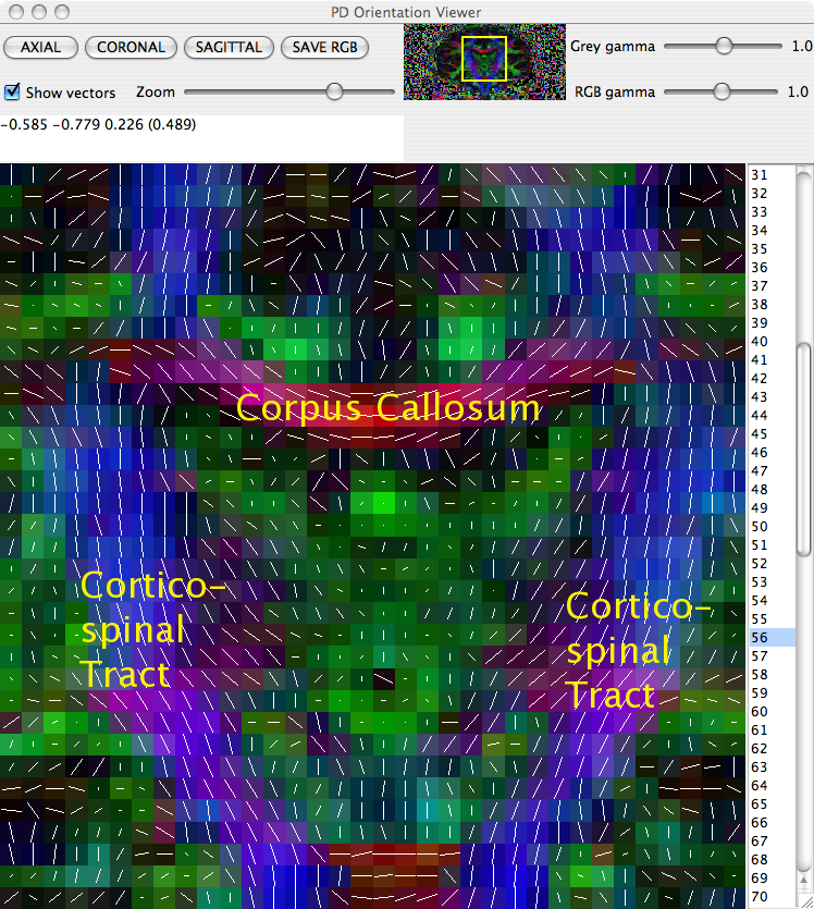
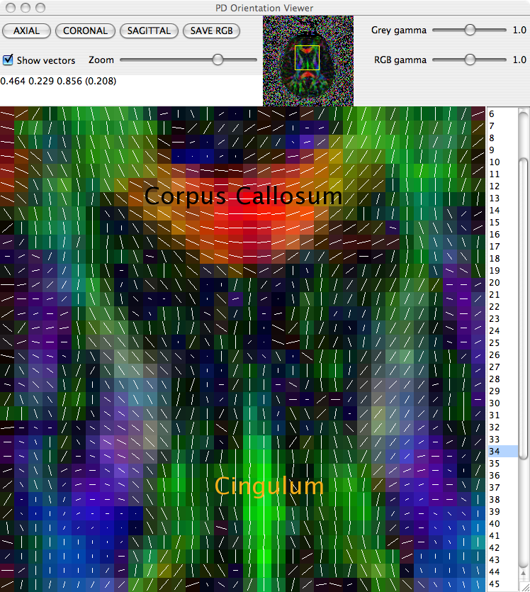
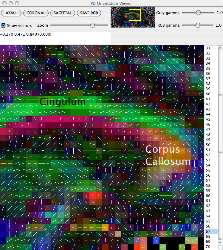
The principal direction of the fitted tensor in each voxel can be directly visualised using the pdview command. This command takes the output of diagonalised tensors and allows a visual check that principal directions are oriented correctly. In the majority of circumstances everything will be fine, but occasionally there can be problems with the data. A common problem is when the coordinate system of the scheme file disagrees with that of the scanner, eg if the z axis in the scheme is -z according to the scanner. If this happens, the anisotropy of tensors will be preserved, but the principal directions will be incorrect.
Because pdview needs the diagonalized tensors rather than the tensors themselves, we must pipe the data through an additional command, dteig that diagonalizes the fitted tensors. A pipeline for visualising principal directions is
cat scans/brainDT.Bdouble | dteig | pdview -datadims 128 128 60
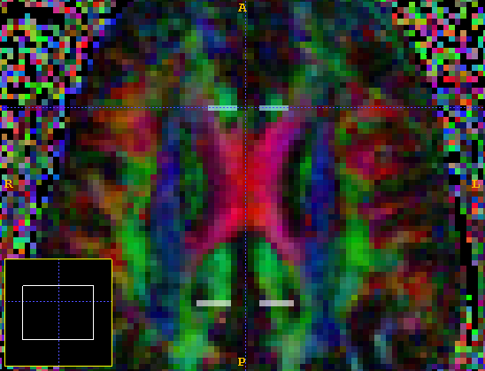
displays a visualisation of the principal direction in each voxel, overlaid on the fractional anisotropy (FA) map. Careful inspection of the directions in regions of the scan in which the principal direction is known can reveal any difficulties in the scan.
To identify which (if any) gradient direction might be flipped it is worth checking three different white matter structures in three different views:
The Cortico-spinal tracts in a coronal slice
The Corpus Collosum in an axial slice
The Cingulum in a sagittal slice
Diagonalising all tensors takes about 30 seconds, after which the visualisation will appear.
Seeding tractography
Performing tractography requires that we specify one or more seed points, from which tractography is initiated. The track command supports three different ways of specifying seed locations: by voxel, by spatial location and by a region-of-interest (ROI) image.
To initialise tractography from a particular voxel, use the input flag -seedpointvox i j k where i, j, k are the integer coordinates of the desired seed voxel.
-seedpointvox 64 64 30
specifies voxel (64,64,30) as the seed for tractography.
To initialise tractography from a given spatial location, use the input flag -seedpointmm x y z where x, y, z are the the spatial coordinates of the seed point, given in mm.
-seedpointmm 108.8 108.8 69.0
specifies that tractography begins at the point (108.8, 108.8, 69.0) mm, in image coordinates.
To initialise tractography from an ROI containing more than one voxel, it is possible to specify a region of interest and import the ROI in analyze format. If an ROI is contained in roi.img and roi.hdr then
-seedfile roi
will start tractography from all (positive) non-zero voxels in the analyze format file roi.img. ROIs may be generated using MRIcro (using "export roi as Analyze image") or a similar package.
A convenient way to visualise data for drawing an ROI is to create an FA image to work from. This is done using the fa command
cat scans/brainDT.Bdouble | fa > scans/brainFA.img
and adding an analyze format header using
analyzeheader -datadims 128 128 60 -voxeldims 1.7 1.7 2.3 -datatype double > scans/brainFA.hdr
The FA map created using this data was used to create a Region of Interest (ROI) using MRIcro which is then used to seed both streamline and probabilistic tractography.
Generating the FA map from the fitted tensors takes about 10 seconds.
Output formats
track is able to produce output results in several different formats, these are specified by using the -outputtracts fmt where fmt is one of: raw (the default), oogl, OOGL format suitable for visualisers such as geomview and voxels which output the voxel coordinates of all points on each track. The specification of the output formats are detailed in the man page track(1).
The filename for results files has the argument of -outputroot (filename) appended to the beginning. -outputroot scans/tracts causes a file called tracts1.oogl to be placed in the scans/ directory. Finally, by specifying the -gzip flag, output will be compressed.
Streamline tractography
We can perform streamline tractography on the fitted tensor data using the track command. Track accepts either tensor or principal direction data. Here we concentrate on tensor tractography. In addition to the data, track needs to know voxel dimensions (in mm), the dimensions of the data in voxels, and also information regarding seed points for the tracks. Since we are using an Analyze ROI to define the seeds, the voxel and data dimensions are read from the Analyze header. A complete streamline tractography pipeline is
cat scans/brainDT.Bdouble | track -inputmodel dt -seedfile roi -outputroot scans/tracts
We have piped in the fitted tensor data from dtfit (or modelfit), specifying the input model as diffusion tensor. We've also specified (via the Analyze header) that the data are arranged in a 128x128x60 grid of 1.7mm x 1.7mm x 2.3mm voxels. The default output type, which we use here, is raw binary. See the track man page for a definition of the file format. The output file will be called tracts1.Bfloat..
In order to visualize the data, we shall convert the streamlines to OOGL format with the procstreamlines command.
cat scans/tracts1.Bfloat | procstreamlines -outputtracts oogl -outputfile scans/tracts1.oogl
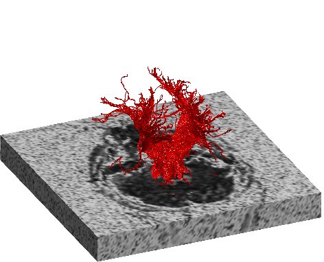
Below are the results of fibre-tracking using the given data and ROI:
These were visualised using Geomview, with the command
geomview scans/tracts1.oogl
In addition to these options we can also specify other parameters relevant to tractography. For example, -ipthresh can be used to specify the track curvature threshold and -stepsize specifies the length of a step through the diffusion tensor field. An anisotropy threshold may be specified with the -anisthresh option. For further options see the track man page.
A Matlab program for streamline visualization is available for download here (tar archive, extract the contents to a directory on Matlab's path). This program was kindly provided by Mara Cercignani, Institute of Neurology, UCL. It reads streamlines in raw binary format, which in our case is the file tracts1.Bfloat. We render these with the Matlab command:
>> plot_streamlines('r', 'scans/tracts1.Bfloat', [1.7 1.7 2.3]);
This process is rather slow (approximately 1 second per streamline). The first argument is the colour of the streamline (we use red), the second argument is the output from track, and the third argument is an array containing the voxel dimensions of the image. After rendering is complete, we make the tracts appear shiny with the command camlight. Finally, we display the FA volume computed above in the same space as the streamlines.
>> add_mri2('scans/brainFA.img',15,'Ax',[128 128 60],'double');
This command loads the FA map, cut at slice 15 in the axial plane. The last two arguments are the data dimensions and the data type of the FA image. The rendered streamlines are shown below.
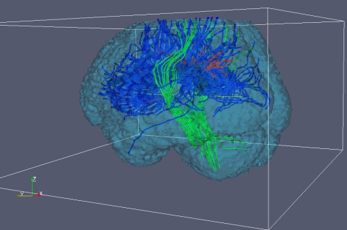
A third option for streamline visualization to to convert the raw streamlines to VTK format with the vtkstreamlines command. This program outputs VTK polylines, which can be loaded into VTK visualization programs such as Paraview. An example image is shown below.
Streamline tracking with two ROIs
Two-ROI tractography is designed to reduce errors by defining two ROIs and finding the paths that intersect both. Camino defines an ROI as all voxels in a seed file with the same nonzero intensity (they need not be contiguous).
Streamlines that do not connect the structures of interest, or that follow erroneous paths, are unlikely to connect both ROIs, and hence are discarded from the analysis. For this section we shall use ITK-SNAP, which has more sophisticated ROI drawing tools than MRICro. We define the ROIs on the color-coded FA map, which we get with the command
dteig -inputfile scans/brainDT.Bdouble | rgbscalarimg -datadims 128 128 60 -voxeldims 1.7 1.7 2.3 -outputroot c1_rgb
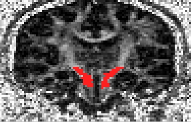
This creates the MetaImage file c1_rgb.mhd. We then draw an ROI at both ends of the cingulum. The posterior ROI is label 1 and the anterior ROI is label 2. We next go to File -> Save Data -> Segmentation Data and save the file as an Analyze volume cingulum2roi.hdr. An axial view of the ROIs from SNAP is shown below.
To get all streamlines seeded in both ROIs, we do
cat scans/brainDT.Bdouble | track -inputmodel dt -seedfile roi -outputroot scans/cing -outputtracts oogl -ipthresh 0.5 -anisthresh 0.1
geomview scans/cing1.oogl scans/cing2.oogl@@
To remove streamlines that don't pass through both ROIs, we pass the seed file to procstreamlines as a "waypoint file". For every positive integer intensity value that exists in the waypoint file (1 and 2 in our case), streamlines must enter at least one voxel with that intensity value. Otherwise, procstreamlines discards them. Note that we output from track to stdout here, and output raw format tracts (procstreamlines reads raw or voxel input, but not OOGL). We run
cat scans/brainDT.Bdouble | track -inputmodel dt -seedfile roi -ipthresh 0.5 -anisthresh 0.1 | procstreamlines -seedfile cingulum2roi.hdr -waypointfile cingulum2roi.hdr -outputroot cing2roi -outputtracts oogl
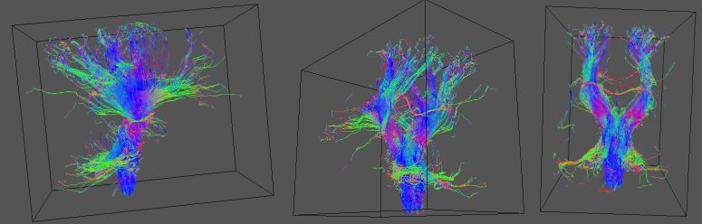
The images below show scans/cing1.oogl and scans/cing2.oogl on the left, and scans/cing2roi1.oogl and scans/cing2roi2.oogl on the right. We see on the left that our ROIs include part of the corpus callosum, but streamlines in the corpus callosum do not intersect both ROIs, so they are missing in the image on the right.
More filtering options with procstreamlines
The procstreamlines command above read tracts from the standard input and output them to two files, one for each ROI. Some equivalent commands are:
cat scans/brainDT.Bdouble | track -inputmodel dt -seedfile roi -ipthresh 0.5 -anisthresh 0.1 -outputroot scans/cingtracts
cat scans/cingtracts1.Bfloat scans/cingtracts2.Bfloat | procstreamlines -seedfile cingulum2roi.hdr -waypointfile cingulum2roi.hdr -outputroot cing2roi -outputtracts oogl
The above command saves the output of track to disk, which is not terribly useful in this example, but would be useful if we hadf spent a long time tracking and wanted to process the same set of streamlines in different ways. We could also do
cat scans/brainDT.Bdouble | track -inputmodel dt -seedfile roi -ipthresh 0.5 -anisthresh 0.1 | procstreamlines -seedfile cingulum2roi.hdr -waypointfile cingulum2roi.hdr -outputtracts oogl > cing2roi
Without the -outputroot option, the output is to stdout. If an output root is specified, output is split by ROI.
track and procstreamlines process tracts in the same order. Let seedImage(x,y,z) be a function that returns the intensity of the seed image for voxel x,y,z. Then:
  for (all rois numbered r) {
            for (all z) {
                for (all y) {
                    for (all x) {
                        s = seedImage(x,y,z);
                        if (s == r) {
                            for (all iterations i) {
                                 track / proces  streamline  for  seed (x,y,z)
                            }
                        }
                   }
                }
            }
  }
For streamline tracking, the number of iterations is 1, for probabilistic tractography (see below) the default is 5000.
Probabilistic Tractography
Camino also implements probabilistic tractography via the PICo algorithm [1][2][3]. Tractography using PICo requires an extra stage in the reconstruction. We generate a look-up table from the schemefile and the signal-to-noise ratio (SNR) of the unweighted (q=0) data. Look-up tables for PICo are generated using the dtlutgen command
dtlutgen -schemefile scans/tensorPoints.scheme -snr 16.0 -inversion 1 -trace 2.1E-9 > scans/picoTable.dat
In addition to the schemefile, we have specified an SNR of 16 and diffusion tensor inversion through the -inversion flag, which takes the same arguments as when used in modelfit. A look-up table needs to be generated once for each scheme, SNR and inversion type.
PICo tractography requires an estimate of the fibre direction and a model of its uncertainty in each voxel.Thee picopdfs command maps PDF parameters from the look-up table to the data
picopdfs -inputmodel dt -luts scans/picoTable.dat
We have specified a diffusion tensor input model and the look-up table generated by the dtlutgen command.
A command pipeline for PICo tractography is then
cat scans/brainDT.Bdouble | picopdfs -inputmodel dt -luts scans/picoTable.dat | track -inputmodel pico -seedfile roi | procstreamlines -seedfile roi -outputcp -outputroot scans/pico/
We have piped the fitted tensor data in the file brainDT.Bdouble into picopdfs and then taken the output of picopdfs and piped it into track, which performs the tractography. We have specified that track should expect PICo input data using the -inputmodel pico flag. By default, track will do 5000 iterations when the input model is pico. If you have many seed points, you may have to reduce this number, but we would not recommend going below 1000. The -outputcp option to track tells it to produce PICo maps. When the -outputcp option is used, procstreamlines assumes PICo tractography, so it will expect 5000 iterations unless told otherwise.
The output of this pipeline is a set of connection probability images in the directory given by the -outputroot option. track has produced one image in analyze format for each seed voxel in the ROI. The final step in producing a coherent connection probability map for the ROI is to combine these images together into a single map for the entire ROI.
This is done using the maxcp command, or equivalently the cpstats command.
maxcp scans/pico/1_ scans/roiprobs
will produce an image of maximum connection probability across each voxel in the ROI. The first argument is the input root for the data, which is the path to the images plus the extra "1_". procstreamlines outputs files named ${outputroot}${region}_${seed}_${pd}.[hdr,img]. In this case, the only region is 1, because there is only 1 ROI in the seed file. The value ${pd} is 1, the default, because there is only one principal direction at each seed point (if there were more, a separate map would exist for each pd).
Combining the results of the separate images into a single maximum connection prob image takes about 25 mins.
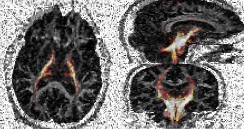
Below are results from PICo tractography:
This image was produced using MRIcro to visualise an FA map from the DT data with the combined probability image scans/roiprobs.hdr(.img) overlayed by using the "Load image overlay..." option from the "Overlay" menu.
For additional options relating to the PICo algorithm, please see the track and procstreamlines man pages.
Performing PICo tractography over the ROI of 898 voxels used in streamline tractography takes around 3.5 hours.
Parallel tracking
The tractography can be performed in parallel by processing each seed point individually. We first save the output of picopdfs to disk:
cat scans/brainDT.Bdouble | picopdfs -inputmodel dt -luts scans/picoTable.dat > brainPICoPDFs.Bdouble
We then count the number of seeds within the seed image:
countseeds roi
This outputs the number of seed voxels in the image roi.img (898). We can perform PICo tractography for a single seed point in the ROI by passing the -seedindex option to track and procstreamlines. For example, to track the first seed, we do:
track -inputfile brainPICoPDFs.Bdouble -inputmodel pico -seedfile roi -seedindex 1 | procstreamlines -outputcp -outputroot scans/pico/ -seedindex 1 \\
When we use -seedindex with the -outputcp option, track names the output files to be consistent with serial processing. The procedure is unchanged if there are multiple ROIs in the seed file.
It is also possible to parallelize tracking by region, using the -regionindex option in place of the -seedindex. All seeds within a specific region are processed together. This may be efficient if you have many regions within the seed file, because we only need to initialize the programs and read in the PICo PDFs once per region, rather than once per seed.
References
[1] Parker et al JMRI 18 (2003) 242-254
[2] Parker & Alexander LNCS 2732 (2003) 684-695
[3] Cook et al LNCS 3749 (2005) 164-171