Camino | Tutorials / ActiveAxTutorial

This tutorial demonstrates ActiveAx - Axon diameter and density estimation and mapping. The algorithm is explained in detail in (Alexander et al NeuroImage 52 (4), 1374-1389, 2010). Please cite that paper and the usual Camino ISMRM abstract if you use this.

This tutorial runs through an example estimating an axon diameter index map from a single data set, which you can download from the DRCMR website here: http://dig.drcmr.dk. This is one of the fixed monkey brain data sets used in (Alexander et al NeuroImage 2010); it is the one in figure 12 (g) and (h). The published results actually used a matlab implementation of the fitting algorithm. The Camino implementation is similar but not identical so minor variations occur. The main difference is longer MCMC, which improves convergence and ameliorates to some extent the overestimation of the axon diameter index that we originally reported. Also the experiment in the NeuroImage paper smoothed the data before fitting and we do not do that here. The smoothing is necessary for the in-vivo data presented in the same paper, but not for the ex-vivo data we use here. In the paper, we smoothed the fixed-brain data mainly for consistency with the in-vivo data. If you want the matlab smoothing code, please email the authors of the paper.

From the DIG homepage, go to the downloads page and download the ActiveAx data set. You may need to register to access the data.

You should have the following files:

DRCMR_ActiveAx4CCfit_E2503_Mbrain1_B13183_3B0_ELEC_N90_Scan1_DIG.nii.gz
DRCMR_ActiveAx4CCfit_E2503_Mbrain1_B1931_3B0_ELEC_N90_Scan1_DIG.nii.gz
DRCMR_ActiveAx4CCfit_E2503_Mbrain1_B1925_3B0_ELEC_N90_Scan1_DIG.nii.gz
DRCMR_ActiveAx4CCfit_E2503_Mbrain1_B3091_3B0_ELEC_N90_Scan1_DIG.nii.gz

You will also need the following files:

ActiveAxG140_PM.scheme1 - the scheme file for the ActiveAxG140 protocol.

MidSagCC.img and MidSagCC.hdr - region of interest outlining the mid-sagital corpus callosum.

''Note on acquisition protocol: The model fitting procedure here does not rely on using the exact protocol defined in ActiveAxG140_PM.scheme1. You can replace that scheme file with your own. However, for sensitivity to the parameters of the MMWMD model, you need to use a multi-shell HARDI acquisition protocol. Moreover, for good sensitivity, the diffusion time should vary between the shells. Just varying the b-value without varying the diffusion time is less likely to produce good results, although we have not tested it.''

Here are the bash commands to run:

# Unzip the data files.
gunzip *.gz

# Add the Camino bin directory to the path
export PATH=${PATH}:~/Camino/camino/bin

# Convert nifti file to Camino format.  Note the header is at the
# start of the file, so we need to strip it off using tail.
export XSIZE=128;
export YSIZE=256;
export ZSIZE=3;
export COMPONENTS=93;

# The input data is little endian shorts so 2 bytes per voxel
# and we need to switch the ordering using shredder.
for i in DRCMR*.nii; do
  tail -c $((XSIZE*YSIZE*ZSIZE*COMPONENTS*2)) $i > ${i%%.nii}.img
done
cat DRCMR*.img | shredder 0 -2 0 | scanner2voxel -voxels $((XSIZE*YSIZE*ZSIZE)) -components $((COMPONENTS*4)) \
-inputdatatype short > All.Bfloat
rm DRCMR*.img

# Run the fitting
modelfit -fitmodel mmwmdfixed -fitalgorithm mcmc -burnin 1000 -samples 100 -interval 500 -noisemodel rician -sigma 200 \
-inputfile All.Bfloat -bgmask MidSagCC.img -schemefile ActiveAxG140_PM.scheme1 | chunkstats -chunksize 16 \
-samples 100 -mean > AllMMWMD_PM.Bdouble

This takes a few hours to run.

Clearly the above needs adapting for other data sets. Adaptations to the data preparation steps should be self explanatory. For the actual model fitting command, the choice of sigma is important and should reflect the standard deviation of the noise in the data. You can estimate it by looking at the standard deviation in the b=0 image; see camino command datastats.

For in-vivo data, you should replace the -fitmodel mmwmdfixed with -fitmodel mmwmdinvivo and replace -chunksize 16 with -chunksize 15. Various other options for the choice of model, fitting algorithm and noise model are available. See man page for modelfit.

Now we can create individual parameter maps. First let's create an FA image to overlay the axon diameter map:

dtfit All.Bfloat ActiveAxG140_PM.scheme1 > AllDT.Bdouble
fa -outputdatatype float < AllDT.Bdouble > AllFA.img
analyzeheader -datadims 128 256 3 -voxeldims 0.4 0.4 2.4 -datatype float > AllFA.hdr

The output file AllMMWMD_PM.Bdouble contains 16 values per voxel. They are:

1. Exit code indicating success/failure of the fitting procedure. 0 means OK. -1 means background. Anything else indicates a problem.
2. S0 - the signal with no diffusion weighting.
3. f1 - the intra-axonal volume fraction (restricted compartment).
4. f2 - the extra-axonal white matter volume fraction (hindered compartment).
5. f3 - the "stationary water" volume fraction.
6. f4 - the CSF volume fraction.
7. d - the intrinsic diffusivity of intra-axonal water. Fixed to 6E-10 m^2/s.
8. theta - angle of colatitude of axon orientation.
9. phi - angle of longitude of axon orientation.
10. R - the axon radius index.
11. d - the parallel diffusivity of the hindered compartment. Fixed to 6E-10 m^2/s.
12. theta - angle of colatitude of principal direction of hindered diffusion (constrained equal to axon orientation).
13. phi - angle of longitude of principal direction of hindered diffusion (constrained equal to axon orientation).
14. d_tort - tortuous diffusivity of perpendicular hindered compartment (constrained to f2*d/(f1+f2)).
15. d_csf - CSF diffusivity. Fixed to 2E-9 m^2/s.
16. f_opt - the fitting residual, here averaged over all MCMC samples.

Thus for a map of axon radius index (note you need to divide by two to get an axon diameter index map as in the NeuroImage paper), we need to extract the tenth value from each voxel. We can do that using shredder:

shredder $((9*8)) 8 $((15*8)) < AllMMWMD_PM.Bdouble > Rad.img
analyzeheader -datadims 128 256 3 -voxeldims 0.4 0.4 2.4 -datatype double > Rad.hdr

Now you can load the FA image into a viewer and overlay the axon radius index map. Here is a snapshot from itksnap showing such an overlay after adjusting the contrast a bit to show the variation.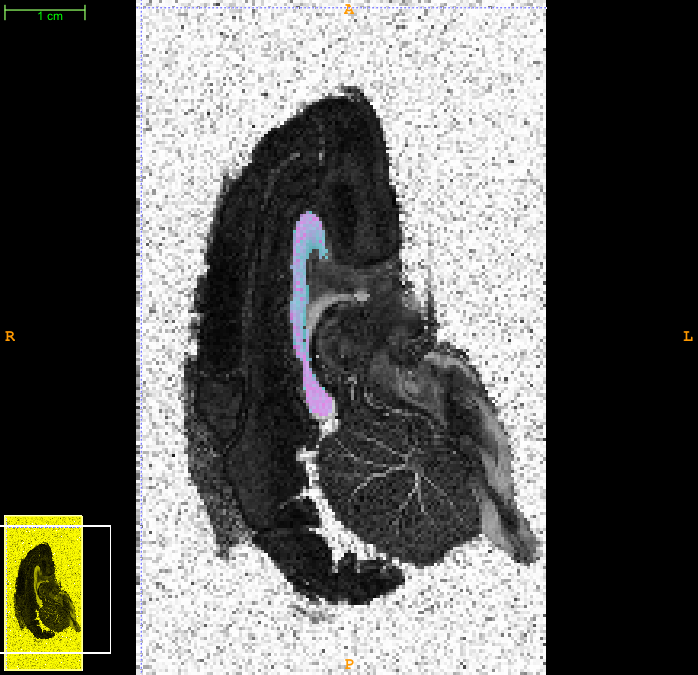

Thresholding and smoothing

The processing pipeline in (Alexander et al NeuroImage 52 (4), 1374-1389, 2010) identifies all voxels with coherent white matter and minimal partial volume with CSF organized by thresholding linearity, planarity and b=0 signal maps. Matlab code for performing those operations is below, but first we need to generate some simple parameter maps using Camino:

# Compute measures of linearity and planarity
dtfit All.Bfloat ActiveAxG140_PM.scheme1 > /tmp/AllDT.Bdouble
dteig < /tmp/AllDT.Bdouble > /tmp/AllDT_EIG.Bdouble
dtshape -stat cl -outputdatatype float < /tmp/AllDT_EIG.Bdouble > AllLin.img
analyzeheader -datadims 128 256 3 -voxeldims 0.4 0.4 2.4 -datatype float > AllLin.hdr
dtshape -stat cp -outputdatatype float < /tmp/AllDT_EIG.Bdouble > AllPlan.img
analyzeheader -datadims 128 256 3 -voxeldims 0.4 0.4 2.4 -datatype float > AllPlan.hdr

# Compute file of DT principal directions
shredder 8 24 72 </tmp/AllDT_EIG.Bdouble > AllPD.Bdouble

Here is the matlab code to do the smoothing: Monkey2503_Smooth.m. You will also need a whole brain binary image mask; here is mine: WholeBrain.img, WholeBrain.hdr.

The matlab script outputs a file WholeBrainL06P02B02000_D90_SmthW2_All.Bfloat, which we run the model fitting on in exactly the same way:

# Run the fitting
modelfit -fitmodel mmwmdfixed -fitalgorithm mcmc -burnin 1000 -samples 100 -interval 500 -noisemodel rician -sigma 200 \
-inputfile WholeBrainL06P02B02000_D90_SmthW2_All.Bfloat -schemefile ActiveAxG140_PM.scheme1 \
-bgmask WholeBrainL06P02B02000_D90_SmthW2_Mask.img | chunkstats -chunksize 16 -samples 100 -mean \
> WholeBrainL06P02B02000_D90_SmthW2_AllMMWMD_PM_Mean.Bdouble &

# Extract the axon radius index file
shredder $((9*8)) 8 $((15*8)) < WholeBrainL06P02B02000_D90_SmthW2_AllMMWMD_PM_Mean.Bdouble > WholeBrainL06P02B02000_D90_SmthW2_Rad.img
analyzeheader -datadims 128 256 3 -voxeldims 0.4 0.4 2.4 -datatype double > WholeBrainL06P02B02000_D90_SmthW2_Rad.hdr

The modelfit command takes a few days to run on a single processor, but you can split it up and run separate chunks on separate processors.

Here is the overlay for the middle slice: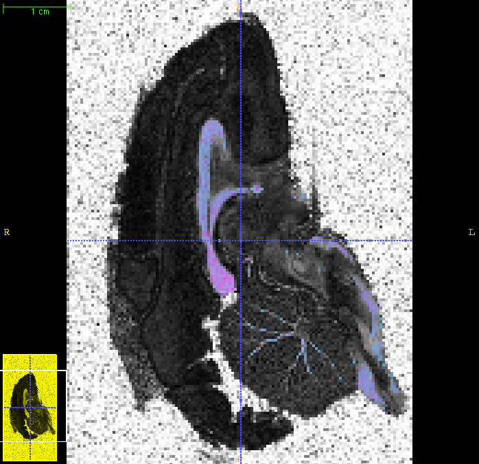

Simulations and testing

This section shows how to repeat the simulation experiments in (Alexander et al NeuroImage 2010) using the Monte Carlo simulation system in (Hall et al IEEE Trans. Med. Im. 2009). Please cite both those papers if you use these ideas in your work.

We find the best-fit gamma distributions to each of the five axon diameter distributions presented in figure 4 of (Aboitiz et al Brain Research 1992) and the six distributions in figure 7 of (Lamantia et al Comp. Neurol. 1990); this requires measuring manually the height of each bin in each histogram and fitting the gamma parameters to the resulting data. Fortunately, we've done it for you. The best-fit gamma parameters, for the Aboitiz histograms (top to bottom of figure 4), divided by two to get distributions of radii rather than diameters, are: (5.3316, 1.0242E-7), (3.5027, 1.6331E-7), (2.8771, 2.4932E-7), (3.2734, 2.4563E-7), and (4.8184, 1.3008E-7); the first number is the shape parameter and the second is the scale parameter. The best-fit gamma parameters for the Lamantia histograms (top to bottom of figure 7), again divided by two, are: (5.9242, 5.3249E-8), (5.2357, 9.3946E-8), (5.2051, 1.0227E-7), (8.5358, 3.7369E-8), (10.196, 3.6983E-8), and (16.275, 1.4282E-8). The simulation experiment in (Alexander et al NIMG 2010) uses each of these distributions as well as distributions in which the size of each cylinder is doubled, which we achieve simply by doubling each scale parameter.

The datasynth command is the access point for the Monte Carlo simulation. The following command runs a simulation within a substrate consisting of 100 packed cylinders with radii drawn from a gamma distribution with shape parameter GAMA and scale parameter GAMB:

datasynth -walkers ${WALKERS} -tmax ${TIMESTEPS} -geometry inflammation -numcylinders 100 -p 0.0 -initial uniform -voxels 1 \
-increments 1 -separateruns -latticesize ${LATSIZE} -schemefile ${SCHEMEFILE} -gamma ${GAMA} ${GAMB} -diffusivity ${DIFF} \
> ${OUTPUTDIR}/${FNAME}

We find that setting WALKERS=160000 and TIMESTEPS=5000 gives good reproducibility and manageable computation times of about 8 hours per run. You can speed things up by reducing these values and sacrificing some accuracy; keep the ratio WALKERS:TIMESTEPS about the same. The lattice size variable LATSIZE determines the packing density of the cylinders: the larger LATSIZE the greater the area we have to pack the cylinders in so the lower the intra-cylinder volume fraction. If LATSIZE is too low, the algorithm cannot pack all the cylinders into the available space. When that happens datasynth will give a warning like this:

Jun 25, 2011 3:04:05 PM simulation.dynamics.StepGeneratorFactory getStepGenerator
INFO: instantiating fixed length step generator
Jun 25, 2011 3:04:06 PM simulation.geometry.substrates.SquashyInflammationSubstrate <init>
WARNING: could only place 46 of 100 cylinders on substrate
Jun 25, 2011 3:04:06 PM simulation.geometry.substrates.SquashyInflammationSubstrate <init>
INFO: intracellular volume fraction 0.6538004810678155
:

To maximize the packing density, you need to tune the LATSIZE variable to find the lowest setting that does not give a warning like that above, ie it packs all 100 cylinders in. Note that you do not need to complete the run of the simulation, as the warning comes out at the start before the time counter starts from 0.0%. The command also outputs the intra-cylinder volume fraction, as shown above.

In the simulations in the paper, we use two settings of the lattice size for each substrate to provide separate simulations with different packing densities. The first lattice size is the lowest value the algorithm packs all 100 cylinders in successfully; the second produces an intracylinder volume fraction about 0.1 less than the first. Since we have 11 different original distributions (5 from Aboitiz; 6 from Lamantia) and we add an extra 11 with each diameter distribution doubled, including two packing densities for each leads to a total of 44 simulations. Here is the full set of datasynth runs we use to synthesize all 44 sets of signals:

#!/bin/bash

SCHEMEFILE=ActiveAxG140_PM.scheme1

WALKERS=160000
TIMESTEPS=5000

DIFF=6.0E-10;

OUTPUTDIR=AbLamSim
mkdir ${OUTPUTDIR}

# Lamantia distributions with diameters doubled

# These are the intra-cylinder volume fractions for each lattice size.
# f1=0.743, f2=0.6061.
LATSIZE=1.4E-5
GAMA=5.9242
GAMB=1.065E-7
FNAME=LamD1a.Bfloat
datasynth -walkers ${WALKERS} -tmax ${TIMESTEPS} -geometry inflammation -numcylinders 100 -p 0.0 -initial uniform -voxels 1 \
-increments 1 -separateruns -latticesize ${LATSIZE} -schemefile ${SCHEMEFILE} -gamma ${GAMA} ${GAMB} -diffusivity ${DIFF} \
> ${OUTPUTDIR}/${FNAME}

LATSIZE=1.55E-5
GAMA=5.9242
GAMB=1.065E-7
FNAME=LamD1b.Bfloat
datasynth -walkers ${WALKERS} -tmax ${TIMESTEPS} -geometry inflammation -numcylinders 100 -p 0.0 -initial uniform -voxels 1 \
-increments 1 -separateruns -latticesize ${LATSIZE} -schemefile ${SCHEMEFILE} -gamma ${GAMA} ${GAMB} -diffusivity ${DIFF} \
> ${OUTPUTDIR}/${FNAME}


# f1=0.7432, f2=0.666.
LATSIZE=2.66E-5
GAMA=5.2357
GAMB=1.8789E-7
FNAME=LamD2a.Bfloat
datasynth -walkers ${WALKERS} -tmax ${TIMESTEPS} -geometry inflammation -numcylinders 100 -p 0.0 -initial uniform -voxels 1 \
-increments 1 -separateruns -latticesize ${LATSIZE} -schemefile ${SCHEMEFILE} -gamma ${GAMA} ${GAMB} -diffusivity ${DIFF} \
> ${OUTPUTDIR}/${FNAME}

LATSIZE=2.81E-5
GAMA=5.2357
GAMB=1.8789E-7
FNAME=LamD2b.Bfloat
datasynth -walkers ${WALKERS} -tmax ${TIMESTEPS} -geometry inflammation -numcylinders 100 -p 0.0 -initial uniform -voxels 1 \
-increments 1 -separateruns -latticesize ${LATSIZE} -schemefile ${SCHEMEFILE} -gamma ${GAMA} ${GAMB} -diffusivity ${DIFF} \
> ${OUTPUTDIR}/${FNAME}


# f1=0.7585, f2=0.6862.
LATSIZE=2.92E-5
GAMA=5.2051
GAMB=2.0454E-7
FNAME=LamD3a.Bfloat
datasynth -walkers ${WALKERS} -tmax ${TIMESTEPS} -geometry inflammation -numcylinders 100 -p 0.0 -initial uniform -voxels 1 \
-increments 1 -separateruns -latticesize ${LATSIZE} -schemefile ${SCHEMEFILE} -gamma ${GAMA} ${GAMB} -diffusivity ${DIFF} \
> ${OUTPUTDIR}/${FNAME}

LATSIZE=3.07E-5
GAMA=5.2051
GAMB=2.0454E-7
FNAME=LamD3b.Bfloat
datasynth -walkers ${WALKERS} -tmax ${TIMESTEPS} -geometry inflammation -numcylinders 100 -p 0.0 -initial uniform -voxels 1 \
-increments 1 -separateruns -latticesize ${LATSIZE} -schemefile ${SCHEMEFILE} -gamma ${GAMA} ${GAMB} -diffusivity ${DIFF} \
> ${OUTPUTDIR}/${FNAME}


# f1=0.7212, f2=0.5989.
LATSIZE=1.54E-5
GAMA=8.5358
GAMB=7.4738E-8
FNAME=LamD4a.Bfloat
datasynth -walkers ${WALKERS} -tmax ${TIMESTEPS} -geometry inflammation -numcylinders 100 -p 0.0 -initial uniform -voxels 1 \
-increments 1 -separateruns -latticesize ${LATSIZE} -schemefile ${SCHEMEFILE} -gamma ${GAMA} ${GAMB} -diffusivity ${DIFF} \
> ${OUTPUTDIR}/${FNAME}

LATSIZE=1.67E-5
GAMA=8.5358
GAMB=7.4738E-8
FNAME=LamD4b.Bfloat
datasynth -walkers ${WALKERS} -tmax ${TIMESTEPS} -geometry inflammation -numcylinders 100 -p 0.0 -initial uniform -voxels 1 \
-increments 1 -separateruns -latticesize ${LATSIZE} -schemefile ${SCHEMEFILE} -gamma ${GAMA} ${GAMB} -diffusivity ${DIFF} \
> ${OUTPUTDIR}/${FNAME}


# f1=0.6897, f2=0.5877.
LATSIZE=1.8E-5
GAMA=10.196
GAMB=7.3966E-8
FNAME=LamD5a.Bfloat
datasynth -walkers ${WALKERS} -tmax ${TIMESTEPS} -geometry inflammation -numcylinders 100 -p 0.0 -initial uniform -voxels 1 \
-increments 1 -separateruns -latticesize ${LATSIZE} -schemefile ${SCHEMEFILE} -gamma ${GAMA} ${GAMB} -diffusivity ${DIFF} \
> ${OUTPUTDIR}/${FNAME}

LATSIZE=1.95E-5
GAMA=10.196
GAMB=7.3966E-8
FNAME=LamD5b.Bfloat
datasynth -walkers ${WALKERS} -tmax ${TIMESTEPS} -geometry inflammation -numcylinders 100 -p 0.0 -initial uniform -voxels 1 \
-increments 1 -separateruns -latticesize ${LATSIZE} -schemefile ${SCHEMEFILE} -gamma ${GAMA} ${GAMB} -diffusivity ${DIFF} \
> ${OUTPUTDIR}/${FNAME}


# f1=0.6525, f2=0.5053
LATSIZE=1.1E-5
GAMA=16.275
GAMB=2.8563E-8
FNAME=LamD6a.Bfloat
datasynth -walkers ${WALKERS} -tmax ${TIMESTEPS} -geometry inflammation -numcylinders 100 -p 0.0 -initial uniform -voxels 1 \
-increments 1 -separateruns -latticesize ${LATSIZE} -schemefile ${SCHEMEFILE} -gamma ${GAMA} ${GAMB} -diffusivity ${DIFF} \
> ${OUTPUTDIR}/${FNAME}

LATSIZE=1.25E-5
GAMA=16.275
GAMB=2.8563E-8
FNAME=LamD6b.Bfloat
datasynth -walkers ${WALKERS} -tmax ${TIMESTEPS} -geometry inflammation -numcylinders 100 -p 0.0 -initial uniform -voxels 1 \
-increments 1 -separateruns -latticesize ${LATSIZE} -schemefile ${SCHEMEFILE} -gamma ${GAMA} ${GAMB} -diffusivity ${DIFF} \
> ${OUTPUTDIR}/${FNAME}



# Aboitiz distributions with diameters doubled

# f1=0.7659, f2=0.7020
LATSIZE=2.92E-5
GAMA=5.3316
GAMB=2.0484E-7
FNAME=AbD1a.Bfloat
datasynth -walkers ${WALKERS} -tmax ${TIMESTEPS} -geometry inflammation -numcylinders 100 -p 0.0 -initial uniform -voxels 1 \
-increments 1 -separateruns -latticesize ${LATSIZE} -schemefile ${SCHEMEFILE} -gamma ${GAMA} ${GAMB} -diffusivity ${DIFF} \
> ${OUTPUTDIR}/${FNAME}

LATSIZE=3.05E-5
GAMA=5.3316
GAMB=2.0484E-7
FNAME=AbD1b.Bfloat
datasynth -walkers ${WALKERS} -tmax ${TIMESTEPS} -geometry inflammation -numcylinders 100 -p 0.0 -initial uniform -voxels 1 \
-increments 1 -separateruns -latticesize ${LATSIZE} -schemefile ${SCHEMEFILE} -gamma ${GAMA} ${GAMB} -diffusivity ${DIFF} \
> ${OUTPUTDIR}/${FNAME}


# f1=0.7407, f2=0.6712
LATSIZE=2.97E-5
GAMA=3.5027
GAMB=3.2663E-7
FNAME=AbD2a.Bfloat
datasynth -walkers ${WALKERS} -tmax ${TIMESTEPS} -geometry inflammation -numcylinders 100 -p 0.0 -initial uniform -voxels 1 \
-increments 1 -separateruns -latticesize ${LATSIZE} -schemefile ${SCHEMEFILE} -gamma ${GAMA} ${GAMB} -diffusivity ${DIFF} \
> ${OUTPUTDIR}/${FNAME}

LATSIZE=3.12E-5
GAMA=3.5027
GAMB=3.2663E-7
FNAME=AbD2b.Bfloat
datasynth -walkers ${WALKERS} -tmax ${TIMESTEPS} -geometry inflammation -numcylinders 100 -p 0.0 -initial uniform -voxels 1 \
-increments 1 -separateruns -latticesize ${LATSIZE} -schemefile ${SCHEMEFILE} -gamma ${GAMA} ${GAMB} -diffusivity ${DIFF} \
> ${OUTPUTDIR}/${FNAME}


# f1=0.8000, f2=0.6800
LATSIZE=3.78E-5
GAMA=2.8771
GAMB=4.9863E-7
FNAME=AbD3a.Bfloat
datasynth -walkers ${WALKERS} -tmax ${TIMESTEPS} -geometry inflammation -numcylinders 100 -p 0.0 -initial uniform -voxels 1 \
-increments 1 -separateruns -latticesize ${LATSIZE} -schemefile ${SCHEMEFILE} -gamma ${GAMA} ${GAMB} -diffusivity ${DIFF} \
> ${OUTPUTDIR}/${FNAME}

LATSIZE=4.1E-5
GAMA=2.8771
GAMB=4.9863E-7
FNAME=AbD3b.Bfloat
datasynth -walkers ${WALKERS} -tmax ${TIMESTEPS} -geometry inflammation -numcylinders 100 -p 0.0 -initial uniform -voxels 1 \
-increments 1 -separateruns -latticesize ${LATSIZE} -schemefile ${SCHEMEFILE} -gamma ${GAMA} ${GAMB} -diffusivity ${DIFF} \
> ${OUTPUTDIR}/${FNAME}


# f1=0.7543, f2=0.6856
LATSIZE=4.29E-5
GAMA=3.2734
GAMB=4.9127E-7
FNAME=AbD4a.Bfloat
datasynth -walkers ${WALKERS} -tmax ${TIMESTEPS} -geometry inflammation -numcylinders 100 -p 0.0 -initial uniform -voxels 1 \
-increments 1 -separateruns -latticesize ${LATSIZE} -schemefile ${SCHEMEFILE} -gamma ${GAMA} ${GAMB} -diffusivity ${DIFF} \
> ${OUTPUTDIR}/${FNAME}

LATSIZE=4.5E-5
GAMA=3.2734
GAMB=4.9127E-7
FNAME=AbD4b.Bfloat
datasynth -walkers ${WALKERS} -tmax ${TIMESTEPS} -geometry inflammation -numcylinders 100 -p 0.0 -initial uniform -voxels 1 \
-increments 1 -separateruns -latticesize ${LATSIZE} -schemefile ${SCHEMEFILE} -gamma ${GAMA} ${GAMB} -diffusivity ${DIFF} \
> ${OUTPUTDIR}/${FNAME}


# f1=0.7463, f2=0.6129
LATSIZE=2.9E-5
GAMA=4.8184
GAMB=2.6016E-7
FNAME=AbD5a.Bfloat
datasynth -walkers ${WALKERS} -tmax ${TIMESTEPS} -geometry inflammation -numcylinders 100 -p 0.0 -initial uniform -voxels 1 \
-increments 1 -separateruns -latticesize ${LATSIZE} -schemefile ${SCHEMEFILE} -gamma ${GAMA} ${GAMB} -diffusivity ${DIFF} \
> ${OUTPUTDIR}/${FNAME}

LATSIZE=3.2E-5
GAMA=4.8184
GAMB=2.6016E-7
FNAME=AbD5b.Bfloat
datasynth -walkers ${WALKERS} -tmax ${TIMESTEPS} -geometry inflammation -numcylinders 100 -p 0.0 -initial uniform -voxels 1 \
-increments 1 -separateruns -latticesize ${LATSIZE} -schemefile ${SCHEMEFILE} -gamma ${GAMA} ${GAMB} -diffusivity ${DIFF} \
> ${OUTPUTDIR}/${FNAME}



# Lamantia original distributions

# f1=0.743, f2=0.5833
LATSIZE=0.7E-5
GAMA=5.9242
GAMB=5.3249E-8
FNAME=LamR1a.Bfloat
datasynth -walkers ${WALKERS} -tmax ${TIMESTEPS} -geometry inflammation -numcylinders 100 -p 0.0 -initial uniform -voxels 1 \
-increments 1 -separateruns -latticesize ${LATSIZE} -schemefile ${SCHEMEFILE} -gamma ${GAMA} ${GAMB} -diffusivity ${DIFF} \
> ${OUTPUTDIR}/${FNAME}

LATSIZE=0.79E-5
GAMA=5.9242
GAMB=5.3249E-8
FNAME=LamR1b.Bfloat
datasynth -walkers ${WALKERS} -tmax ${TIMESTEPS} -geometry inflammation -numcylinders 100 -p 0.0 -initial uniform -voxels 1 \
-increments 1 -separateruns -latticesize ${LATSIZE} -schemefile ${SCHEMEFILE} -gamma ${GAMA} ${GAMB} -diffusivity ${DIFF} \
> ${OUTPUTDIR}/${FNAME}


# f1=0.7432, f2=0.6002
LATSIZE=1.33E-5
GAMA=5.2357
GAMB=9.3946E-8
FNAME=LamR2a.Bfloat
datasynth -walkers ${WALKERS} -tmax ${TIMESTEPS} -geometry inflammation -numcylinders 100 -p 0.0 -initial uniform -voxels 1 \
-increments 1 -separateruns -latticesize ${LATSIZE} -schemefile ${SCHEMEFILE} -gamma ${GAMA} ${GAMB} -diffusivity ${DIFF} \
> ${OUTPUTDIR}/${FNAME}

LATSIZE=1.48E-5
GAMA=5.2357
GAMB=9.3946E-8
FNAME=LamR2b.Bfloat
datasynth -walkers ${WALKERS} -tmax ${TIMESTEPS} -geometry inflammation -numcylinders 100 -p 0.0 -initial uniform -voxels 1 \
-increments 1 -separateruns -latticesize ${LATSIZE} -schemefile ${SCHEMEFILE} -gamma ${GAMA} ${GAMB} -diffusivity ${DIFF} \
> ${OUTPUTDIR}/${FNAME}


# f1=0.7585, f2=0.6237
LATSIZE=1.46E-5
GAMA=5.2051
GAMB=1.0227E-7
FNAME=LamR3a.Bfloat
datasynth -walkers ${WALKERS} -tmax ${TIMESTEPS} -geometry inflammation -numcylinders 100 -p 0.0 -initial uniform -voxels 1 \
-increments 1 -separateruns -latticesize ${LATSIZE} -schemefile ${SCHEMEFILE} -gamma ${GAMA} ${GAMB} -diffusivity ${DIFF} \
> ${OUTPUTDIR}/${FNAME}

LATSIZE=1.61E-5
GAMA=5.2051
GAMB=1.0227E-7
FNAME=LamR3b.Bfloat
datasynth -walkers ${WALKERS} -tmax ${TIMESTEPS} -geometry inflammation -numcylinders 100 -p 0.0 -initial uniform -voxels 1 \
-increments 1 -separateruns -latticesize ${LATSIZE} -schemefile ${SCHEMEFILE} -gamma ${GAMA} ${GAMB} -diffusivity ${DIFF} \
> ${OUTPUTDIR}/${FNAME}


# f1=0.7212, f2=0.606
LATSIZE=0.77E-5
GAMA=8.5358
GAMB=3.7369E-8
FNAME=LamR4a.Bfloat
datasynth -walkers ${WALKERS} -tmax ${TIMESTEPS} -geometry inflammation -numcylinders 100 -p 0.0 -initial uniform -voxels 1 \
-increments 1 -separateruns -latticesize ${LATSIZE} -schemefile ${SCHEMEFILE} -gamma ${GAMA} ${GAMB} -diffusivity ${DIFF} \
> ${OUTPUTDIR}/${FNAME}

LATSIZE=0.84E-5
GAMA=8.5358
GAMB=3.7369E-8
FNAME=LamR4b.Bfloat
datasynth -walkers ${WALKERS} -tmax ${TIMESTEPS} -geometry inflammation -numcylinders 100 -p 0.0 -initial uniform -voxels 1 \
-increments 1 -separateruns -latticesize ${LATSIZE} -schemefile ${SCHEMEFILE} -gamma ${GAMA} ${GAMB} -diffusivity ${DIFF} \
> ${OUTPUTDIR}/${FNAME}


# f1=0.6897, f2=0.57
LATSIZE=0.9E-5
GAMA=10.196
GAMB=3.6983E-8
FNAME=LamR5a.Bfloat
datasynth -walkers ${WALKERS} -tmax ${TIMESTEPS} -geometry inflammation -numcylinders 100 -p 0.0 -initial uniform -voxels 1 \
-increments 1 -separateruns -latticesize ${LATSIZE} -schemefile ${SCHEMEFILE} -gamma ${GAMA} ${GAMB} -diffusivity ${DIFF} \
> ${OUTPUTDIR}/${FNAME}

LATSIZE=0.99E-5
GAMA=10.196
GAMB=3.6983E-8
FNAME=LamR5b.Bfloat
datasynth -walkers ${WALKERS} -tmax ${TIMESTEPS} -geometry inflammation -numcylinders 100 -p 0.0 -initial uniform -voxels 1 \
-increments 1 -separateruns -latticesize ${LATSIZE} -schemefile ${SCHEMEFILE} -gamma ${GAMA} ${GAMB} -diffusivity ${DIFF} \
> ${OUTPUTDIR}/${FNAME}


# f1=0.6525, f2=0.5483
LATSIZE=0.55E-5
GAMA=16.275
GAMB=1.4282E-8
FNAME=LamR6a.Bfloat
datasynth -walkers ${WALKERS} -tmax ${TIMESTEPS} -geometry inflammation -numcylinders 100 -p 0.0 -initial uniform -voxels 1 \
-increments 1 -separateruns -latticesize ${LATSIZE} -schemefile ${SCHEMEFILE} -gamma ${GAMA} ${GAMB} -diffusivity ${DIFF} \
> ${OUTPUTDIR}/${FNAME}

LATSIZE=0.6E-5
GAMA=16.275
GAMB=1.4282E-8
FNAME=LamR6b.Bfloat
datasynth -walkers ${WALKERS} -tmax ${TIMESTEPS} -geometry inflammation -numcylinders 100 -p 0.0 -initial uniform -voxels 1 \
-increments 1 -separateruns -latticesize ${LATSIZE} -schemefile ${SCHEMEFILE} -gamma ${GAMA} ${GAMB} -diffusivity ${DIFF} \
> ${OUTPUTDIR}/${FNAME}



# Aboitiz original distributions

# f1=0.7256, f2=0.6378
LATSIZE=1.5E-5
GAMA=5.3316
GAMB=1.0242E-7
FNAME=AbR1a.Bfloat
datasynth -walkers ${WALKERS} -tmax ${TIMESTEPS} -geometry inflammation -numcylinders 100 -p 0.0 -initial uniform -voxels 1 \
-increments 1 -separateruns -latticesize ${LATSIZE} -schemefile ${SCHEMEFILE} -gamma ${GAMA} ${GAMB} -diffusivity ${DIFF} \
> ${OUTPUTDIR}/${FNAME}

LATSIZE=1.6E-5
GAMA=5.3316
GAMB=1.0242E-7
FNAME=AbR1b.Bfloat
datasynth -walkers ${WALKERS} -tmax ${TIMESTEPS} -geometry inflammation -numcylinders 100 -p 0.0 -initial uniform -voxels 1 \
-increments 1 -separateruns -latticesize ${LATSIZE} -schemefile ${SCHEMEFILE} -gamma ${GAMA} ${GAMB} -diffusivity ${DIFF} \
> ${OUTPUTDIR}/${FNAME}


# f1=0.7259, f2=0.638
LATSIZE=1.5E-5
GAMA=3.5027
GAMB=1.6331E-7
FNAME=AbR2a.Bfloat
datasynth -walkers ${WALKERS} -tmax ${TIMESTEPS} -geometry inflammation -numcylinders 100 -p 0.0 -initial uniform -voxels 1 \
-increments 1 -separateruns -latticesize ${LATSIZE} -schemefile ${SCHEMEFILE} -gamma ${GAMA} ${GAMB} -diffusivity ${DIFF} \
> ${OUTPUTDIR}/${FNAME}

LATSIZE=1.6E-5
GAMA=3.5027
GAMB=1.6331E-7
FNAME=AbR2b.Bfloat
datasynth -walkers ${WALKERS} -tmax ${TIMESTEPS} -geometry inflammation -numcylinders 100 -p 0.0 -initial uniform -voxels 1 \
-increments 1 -separateruns -latticesize ${LATSIZE} -schemefile ${SCHEMEFILE} -gamma ${GAMA} ${GAMB} -diffusivity ${DIFF} \
> ${OUTPUTDIR}/${FNAME}


# f1=0.8000, f2=0.6867
LATSIZE=1.89E-5
GAMA=2.8771
GAMB=2.4932E-7
FNAME=AbR3a.Bfloat
datasynth -walkers ${WALKERS} -tmax ${TIMESTEPS} -geometry inflammation -numcylinders 100 -p 0.0 -initial uniform -voxels 1 \
-increments 1 -separateruns -latticesize ${LATSIZE} -schemefile ${SCHEMEFILE} -gamma ${GAMA} ${GAMB} -diffusivity ${DIFF} \
> ${OUTPUTDIR}/${FNAME}

LATSIZE=2.04E-5
GAMA=2.8771
GAMB=2.4932E-7
FNAME=AbR3b.Bfloat
datasynth -walkers ${WALKERS} -tmax ${TIMESTEPS} -geometry inflammation -numcylinders 100 -p 0.0 -initial uniform -voxels 1 \
-increments 1 -separateruns -latticesize ${LATSIZE} -schemefile ${SCHEMEFILE} -gamma ${GAMA} ${GAMB} -diffusivity ${DIFF} \
> ${OUTPUTDIR}/${FNAME}


# f1=0.7508, f2=0.656
LATSIZE=2.15E-5
GAMA=3.2734
GAMB=2.4563E-7
FNAME=AbR4a.Bfloat
datasynth -walkers ${WALKERS} -tmax ${TIMESTEPS} -geometry inflammation -numcylinders 100 -p 0.0 -initial uniform -voxels 1 \
-increments 1 -separateruns -latticesize ${LATSIZE} -schemefile ${SCHEMEFILE} -gamma ${GAMA} ${GAMB} -diffusivity ${DIFF} \
> ${OUTPUTDIR}/${FNAME}

LATSIZE=2.3E-5
GAMA=3.2734
GAMB=2.4563E-7
FNAME=AbR4b.Bfloat
datasynth -walkers ${WALKERS} -tmax ${TIMESTEPS} -geometry inflammation -numcylinders 100 -p 0.0 -initial uniform -voxels 1 \
-increments 1 -separateruns -latticesize ${LATSIZE} -schemefile ${SCHEMEFILE} -gamma ${GAMA} ${GAMB} -diffusivity ${DIFF} \
> ${OUTPUTDIR}/${FNAME}


# f1=0.7463, f2=0.6129
LATSIZE=1.45E-5
GAMA=4.8184
GAMB=1.3008E-7
FNAME=AbR5a.Bfloat
datasynth -walkers ${WALKERS} -tmax ${TIMESTEPS} -geometry inflammation -numcylinders 100 -p 0.0 -initial uniform -voxels 1 \
-increments 1 -separateruns -latticesize ${LATSIZE} -schemefile ${SCHEMEFILE} -gamma ${GAMA} ${GAMB} -diffusivity ${DIFF} \
> ${OUTPUTDIR}/${FNAME}

LATSIZE=1.6E-5
GAMA=4.8184
GAMB=1.3008E-7
FNAME=AbR5b.Bfloat
datasynth -walkers ${WALKERS} -tmax ${TIMESTEPS} -geometry inflammation -numcylinders 100 -p 0.0 -initial uniform -voxels 1 \
-increments 1 -separateruns -latticesize ${LATSIZE} -schemefile ${SCHEMEFILE} -gamma ${GAMA} ${GAMB} -diffusivity ${DIFF} \
> ${OUTPUTDIR}/${FNAME}

Running all these commands one after the other takes quite a long time (of order 1 week), but each is independent so you can split them up and run them concurrently on separate processors. Once they are all complete, concatenate them all into a single data file:

cat ${OUTPUTDIR}/AbD* ${OUTPUTDIR}/AbR* ${OUTPUTDIR}/LamD* ${OUTPUTDIR}/LamR* > ${OUTPUTDIR}.Bfloat

Here is the output for schemefile ActiveAxG140_PM.scheme1: AbLamSim.Bfloat.

Now we can run the fitting procedure on the noise free synthetic data (note that we need to set the noise standard deviation -sigma <sig> to an artificial non-zero value for the Rician noise model to work; we pretend here that SNR is 100):

cat AbLamSim.Bfloat | modelfit -fitmodel mmwmdfixed -fitalgorithm mcmc -mmwmddiff 6E-10 -burnin 1000 -samples 100 -interval 500 \
-noisemodel rician -sigma 1600 -schemefile ActiveAxG140_PM.scheme1 | chunkstats -chunksize 16 -samples 100 -mean > AbLamSimMMWMD.Bdouble

We can also generate ten independent noise trials derived from the noise free data, as in (Alexander et al NIMG 2010). We'll generate two: one with SNR at b=0 of 50 and one with SNR or 20. Note that the unweighted signal for the simulations is the number of walkers specified in the datasynth command, so we set the value of sigma to WALKERS/SNR:

for ((i=1; i<=10; i=i+1)); do cat AbLamSim.Bfloat ; done | addnoise -sigma 3200 > AbLamSimT10S002.Bfloat 
for ((i=1; i<=10; i=i+1)); do cat AbLamSim.Bfloat ; done | addnoise -sigma 8000 > AbLamSimT10S005.Bfloat

and run the fitting over the noisy data sets:

cat AbLamSimT10S002.Bfloat | modelfit -fitmodel mmwmdfixed -fitalgorithm mcmc -mmwmddiff 6E-10 -burnin 1000 -samples 100 \
-interval 500 -noisemodel rician -sigma 3200 -schemefile ActiveAxG140_PM.scheme1 | chunkstats -chunksize 16 -samples 100 \
-mean > AbLamSimT10S002_MMWMD.Bdouble
cat AbLamSimT10S005.Bfloat | modelfit -fitmodel mmwmdfixed -fitalgorithm mcmc -mmwmddiff 6E-10 -burnin 1000 -samples 100 \
-interval 500 -noisemodel rician -sigma 8000 -schemefile ActiveAxG140_PM.scheme1 | chunkstats -chunksize 16 -samples 100 \
-mean > AbLamSimT10S005_MMWMD.Bdouble

To test and evaluate the fitted axon diameter index, we need to compute a similar statistic of each axon diameter distribution. We can get the exact list of cylinder radii that make up each substrate, by adding the -substrateinfo@ flag to the datasynth@@ command. For example, for the first substrate in the long list above, we can run:

LATSIZE=1.4E-5
GAMA=5.9242
GAMB=1.065E-7
FNAME=LamD1a.Bfloat
datasynth -walkers 5 -tmax 5 -geometry inflammation -numcylinders 100 -p 0.0 -initial uniform -voxels 1 \
-increments 1 -separateruns -latticesize ${LATSIZE} -schemefile ActiveAxG140_PM.scheme1 -gamma ${GAMA} ${GAMB} \
-diffusivity ${DIFF} -substrateinfo > /tmp/test.Bfloat 2> LamD1a.info

We set the number of walkers and timesteps very low, as we are just interested in the substrate information rather than the output, which we have already computed. The file LamD1a.info contains the position and size of each cylinder:

cylinder 0 pos = (6.65278756664775E-6, 1.8736510967768196E-6, 0.0)      radius = 2.4836106445030362E-6
cylinder 1 pos = (7.075179421691923E-6, 6.310782215503249E-6, 0.0)      radius = 1.2288218199625427E-6
cylinder 2 pos = (9.040679260286337E-7, 1.358410391168818E-5, 0.0)      radius = 1.2057082606855263E-6
cylinder 3 pos = (4.391993962910324E-6, 7.3503496846908985E-6, 0.0)     radius = 1.0606081830751333E-6
cylinder 4 pos = (9.776132252482087E-6, 1.1165129374727735E-5, 0.0)     radius = 1.0479898302635493E-6
cylinder 5 pos = (2.2709875877317475E-7, 2.8099470916851546E-6, 0.0)    radius = 1.0133293909377957E-6
cylinder 6 pos = (9.976382544843197E-6, 1.3158389965085646E-5, 0.0)     radius = 9.45079565714962E-7
cylinder 7 pos = (1.01430033661826E-5, 2.5476110220568397E-6, 0.0)      radius = 9.190732393643317E-7
cylinder 8 pos = (1.2759519960773037E-5, 1.3126264521291948E-5, 0.0)    radius = 9.166534852189462E-7
:
:

Here is a simple perl script to filter out just the list of cylinder radii: ParseSimOutput.pl. Thus,

ParseSimOutput.pl LamD1a.txt

Produces just the list:

2.4836106445030362E-6
1.2288218199625427E-6
1.2057082606855263E-6
1.0606081830751333E-6
1.0479898302635493E-6
1.0133293909377957E-6
9.45079565714962E-7
9.190732393643317E-7
9.166534852189462E-7
:
:

From these lists, we can compute the mean axon diameter 2*(sum of the list / 100), the factor of two converts from radius to diameter, or the mean axon diameter weighted by volume 2*(sum(list.^3)/sum(list.^2)). The latter is close to what we expect for the axon diameter index; see (Alexander et al NIMG 2010) equation 4.

This file: RadInfo.mat, contains an array of mean axon radius meanRad, mean axon radius weighted by volume meanRadByVol, and intra-cylinder volume fractions fs, for each of the 44 substrates in the order they are generated above. It also contains the list of cylinder radii for each substrate. For example, RadListALS_LamD01a contains the same list of radii we obtained from ParseSimOutput.pl LamD1a.txt above.

Here is matlab code to create figures similar to the top left panel in figure 4 of (Alexander et al NIMG 2010) and the left panel of figure 5:

% Load in the fitted parameters from the noise free data.
fid = fopen('AbLamSimMMWMD.Bdouble', 'r', 'b');
res = fread(fid, 'double');
fclose(fid);
noisefreefit = reshape(res, [16,44]);

% Load in the fitted parameters from the noisy data.
fid = fopen('AbLamSimT10S002_MMWMD.Bdouble', 'r', 'b');
res = fread(fid, 'double');
fclose(fid);
noisyfit = reshape(res, [16,440]);

% Load in the ground truth data.
load('RadInfo.mat');

figure; 

% Plot the axon diameter indices
subplot(2,1,1);
hold on;
set(gca, 'FontName', 'Times');
set(gca, 'FontSize', 17);

% Plot the individual noise trials
% We need to double to get diameters from estimated radii.
scatter(2*noisyfit(10,:), 2*repmat(meanRadByVol, [1,10]), 'r', 'SizeData', 50, 'LineWidth', 1);

% Plot the means over the noise trials.
mmps = squeeze(mean(reshape(noisyfit', [44,10, 16]), 2));
scatter(2*mmps(:,10), 2*meanRadByVol, 'bx', 'SizeData', 100, 'LineWidth', 3);

% Now add the noise-free estimates
scatter(2*noisefreefit(10,:), 2*meanRadByVol, 'k', 'SizeData', 100, 'LineWidth', 3);

% Add labels etc
xlabel('a ''/\mum');
ylabel('\alpha/\mum');
xlim([0 7E-6]);
legend('SNR=20', 'E(SNR=20)', 'SNR=\infty', 'Location', 'NorthWest');

% Now plot the volume fractions
subplot(2,1,2);
hold on;
set(gca, 'FontName', 'Times');
set(gca, 'FontSize', 17);

scatter(noisyfit(3,:), repmat(fs, [1,10]), 'r', 'SizeData', 50, 'LineWidth', 1);
scatter(mmps(:,3), fs, 'bx', 'SizeData', 100, 'LineWidth', 3);
scatter(noisefreefit(3,:), fs, 'k', 'SizeData', 100, 'LineWidth', 3);

xlabel('f ''');
ylabel('f');

% Finally output the figure
set(gcf, 'PaperPositionMode', 'manual');
set(gcf, 'PaperUnits', 'inches');
set(gcf, 'PaperPosition', [0 0 4.5 9]);
print -dpng 'AvAlphaFvF.png'

Here is the figure that results: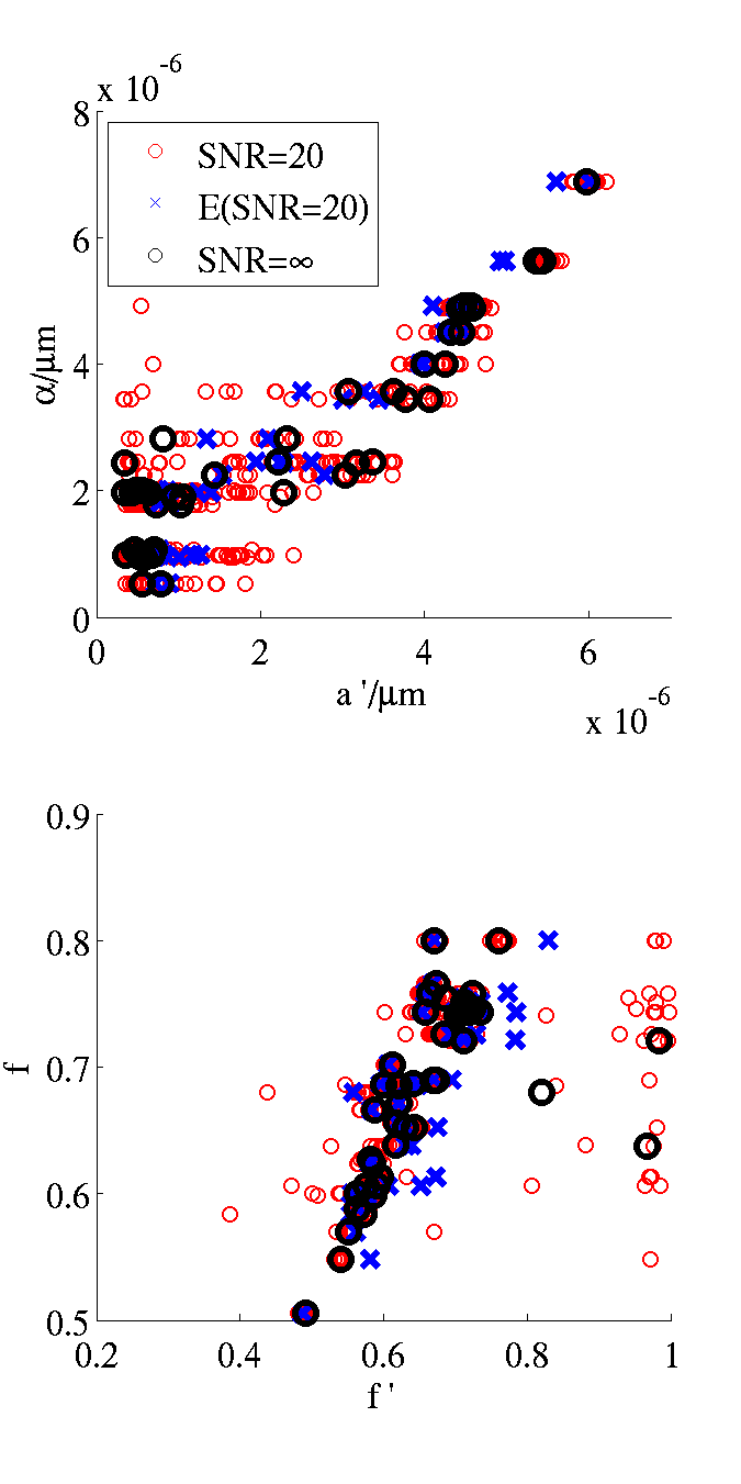

Here is an adaptation of the datasynth command above that outputs the list of cylinders to output also a figure showing a cross section of the substrate used for the simulation (we just add the -drawcrosssection option):

LATSIZE=1.4E-5
GAMA=5.9242
GAMB=1.065E-7
FNAME=LamD1a.Bfloat
datasynth -walkers 5 -tmax 5 -geometry inflammation -numcylinders 100 -p 0.0 -initial uniform -voxels 1 \
-increments 1 -separateruns -latticesize ${LATSIZE} -schemefile ActiveAxG140_PM.scheme1 -gamma ${GAMA} ${GAMB} \
-diffusivity ${DIFF} -substrateinfo -drawcrosssection LamD1aSubstrate.gray > /tmp/test.Bfloat 2> LamD1a.info

The file LamD1aSubstrate.gray contains a simple bitmap which you can display using, for example, ImageMagick as follows:

display -size 500x500 -depth 8 /tmp/xsec.gray

It looks like this: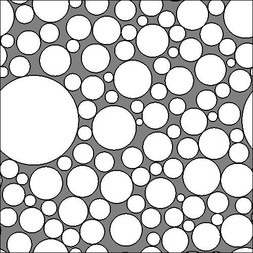

The simulations above all assume that f3 and f4 in the MMWMD model are zero. The (Alexander et al NIMG 2010) paper also contains simulations with those volume fractions set greater than zero. The synthetic data for those simulations comes simply from loading the synthetic data from the Monte Carlo simulation above into matlab and adding a proportion of signal from the model of each of those extra compartments.