Tutorial: Running PASMRI in parallel using SGE
This case study shows how to use a multi-processor cluster running the Sun Grid Engine (SGE) to run PASMRI over a full data set. This case study uses the pig brain data set described and available in the Pig Brain tutorial.
Make sure camino/bin is in your PATH. Download the data file and unpack it:
bunzip2 e1809_15.tar.bz2
tar -xvf e1809_15.tar
Make a voxel-order data file for Camino to work with:
cd e1809_15
cat *.img | shredder 0 -2 0 | scanner2voxel -voxels 163840 -components 64 -inputdatatype short > e1809_15.Bfloat
Check the fitted DT and FA:
dtfit e1809_15.Bfloat e1809_15/e1809_15.scheme > e1809_15_DT.Bdouble
fa < e1809_15_DT.Bdouble > e1809_15_FA.Bdouble
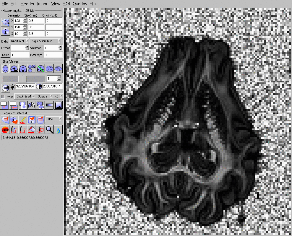
Check the FA map by creating an analyze image:
analyzeheader -voxeldims 0.5 0.5 3.5 -datadims 128 128 10 -datatype double > e1809_15_FA.hdr
cp e1809_15_FA.Bdouble e1809_15_FA.img
Now you can load e1809_15_FA.hdr into MRIcro (for example) and check that it looks like this (click image for full size):
Since PASMRI is a computationally heavy algorithm, we only want to process foreground voxels and not waste time reconstructing in the background. Here we will create background masks via a simple thresholding of the b=0 intensity to segment foreground and background. A better separation can be obtained using, for example, FSL's BET. (The spatial normalization tutorial shows how to do this).
Load the diffusion tensor file into matlab and make a mask by thresholding b=0 intensity at 500:
>> fid = fopen('e1809_15_DT.Bdouble', 'r', 'b');
>> d = fread(fid, 'double');
>> fclose(fid);
>> dt = reshape(d, 8, 128,128,10);
>> mask = exp(dt(2,:,:,:)) > 500;
>> %CHECK THRESHOLD HERE!!!>> fid=fopen('e1809_15_BrainMask.char', 'w', 'b');
>> fwrite(fid, mask, 'char'); \\ >> fclose(fid);
It is convenient to work with separate data files containing each slice when running these big processes on clusters of processors. Here we use the unix command split to split the data set into separate axial slices:
split -b 4194304 e1809_15.Bfloat e1809_15_SLICE
for i in e1809_15_SLICE??; do mv $i $i.Bfloat; done
The commands above create ten files, e1809_15_SLICEaa.Bfloat, e1809_15_SLICEab.Bfloat, ..., e1809_15_SLICEaj.Bfloat, each containing one axial slice of the data set. Split the mask into slices as well:
split -b 16384 e1809_15_BrainMask.char e1809_15_BrainMaskSLICE
for i in e1809_15_BrainMaskSLICE??; do mv $i $i.char; done
The commands for running PASMRI in parallel on a cluster all rely on the Sun Grid Engine, so you'll need that installed on your cluster. Parallel processing is implemented in various scripts in the camino/SGE directory. You need to check and change a few paths to make them appropriate to your setup. First check that the paths to perl, bash and csh are correct at the top of each script in the SGE directory. Also, you'll need to change the path to your camino directory in the variable BASE in the script SGE/PAS_Wrapper.
First, let's try one slice in the middle of the data set to see if everything is working OK.
mkdir PAS_E1809_15
cd camino
SGE/PAS_Submit ../e1809_15/e1809_15_SLICEae.Bfloat ../e1809_15/e1809_15_BrainMaskSLICEae.char 16384 ../e1809_15/e1809_15.scheme 3 ../PAS_E1809_15/e1809_15_SLICEae
The directory PAS_E1809_15 will contain all the results. PAS_Submit submits a separate SGE job for each non-background voxel in the slice. The SGE job runs PASMRI on the data in a voxel and outputs the results in PAS_E1809_15/e1800_15_SLICEae/????????.Bdouble; the directory for the output is specified in the last argument to PAS_Submit and ???????? is the voxel number padded with zeros to eight characters - in the range {00000000, ..., 00016383} in our example. The job also runs sfpeaks on the PAS data to get the peak directions and puts the results in PAS_E1809_15/e1800_15_SLICEae/????????_PDs.Bdouble. For background voxels, PAS_Submit creates output files directly containing default values and does not submit a job to the SGE queue.
After all jobs have completed, each output file ????????.Bdouble should contain N+3 doubles, where N is the number of diffusion weighted measurements. So for the pig brain data, where N=61, each file contains 64 values and so has size 64*8 = 512 bytes. Each ????????_PDs.Bdouble contains 30 doubles (see the sfpeaks man page for details) and so should have size 240 bytes.
Sometimes the occasional process fails or times out leading to missing or empty output files. This command searches for missing or empty output files and resubmits the corresponding jobs.
SGE/PAS_CompleteMissing ../e1809_15/e1809_15_SLICEae.Bfloat ../e1809_15/e1809_15.scheme ../PAS_E1809_15/e1809_15_SLICEae
Finally, this command groups all the single-voxel outputs into a single file containing all the results for the slice in voxel order.
for f in ../PAS_E1809_15/e1809_15_SLICE??; do SGE/CompletePAS $f; echo Done $f; done
The command above replaces the directory PAS_E1809_15/e1809_15_SLICEae and its contents with two files PAS_E1809_15/e1809_15_SLICEae.Bdouble and PAS_E1809_15/e1809_15_SLICEae_PDs.Bdouble, which contain all the PAS results and all the sfpeaks results concatenated, respectively. The size of the the file e1809_15_SLICEae.Bdouble should be 128*128*512 = 8388608 bytes and the size of the file e1809_15_SLICEae_PDs.Bdouble should be 128*128*240 = 3932160 bytes.
Create an axial PAS plot using sfplot to check that everything has worked OK and the results look reasonable. First we need to make an FA map for the slice to use as background for the image:
modelfit -inputfile ../e1809_15/e1809_15_SLICEae.Bfloat -schemefile e1809_15/e1809_15.scheme -bgthresh 500 | fa > /tmp/e1809_15_SLICEae_FA.Bdouble
Now use sfplot (see the sfplot man page for a variety of options you can use to change the appearance of the plot we make here) to generate a nice picture of the PAS function in each voxel of the slice:
sfplot -xsize 128 -ysize 128 -inputmodel maxent -filter PAS 1.4 -mepointset 61 -pointset 2 -minifigsize 30 30 -minifigseparation 2 2 -inputdatatype double -dircolcode -backdrop /tmp/e1809_15_SLICEae_FA.Bdouble -projection 2 1 -colcode 1 2 3 < PAS_E1809_15/e1809_15_SLICEae.Bdouble > /tmp/e1809_15_SLICEae_PAS.rgb
Note the required projection and colour coding. Projection 2 1 says to project each PAS function into the xy-plane, but also to swap the x and y directions of each function, which is necessary because the acquisition swaps then with respect to the image axes. A non-default colour coding is also required, for the same reason, in order to get the familiar colour coding of red for left-right, green for anterior-posterior and blue for superior-inferior. For other data sets, you may need to experiment with these settings to get the orientations right.
Convert the output image to PNG format for economy using the ImageMagick command convert:
convert -size 4096x4096 -depth 8 /tmp/e1809_15_SLICEae_PAS.rgb /tmp/e1809_15_SLICEae_PAS.png;
The output looks like this (click image for full size):
If everything is working OK, submit all the slices:
for f in ../e1809_15/e1809_15_SLICE??.Bfloat; do OFROOT=${f.Bfloat}; OFDIR=${OFROOT##*/}; SLICEID=${OFDIR##*SLICE}; SGE/PAS_Submit $f ../e1809_15/e1809_15_BrainMaskSLICE${SLICEID}.char 16384 ../e1809_15/e1809_15.scheme 3 ../PAS_E1809_15/$OFDIR; done
Check for any missing output files:
for f in ../e1809_15/e1809_15_SLICE??.Bfloat; do OFROOT=${f.Bfloat}; OFDIR=${OFROOT##*/}; SGE/PAS_CompleteMissing $f ../e1809_15/e1809_15.scheme ../PAS_E1809_15/$OFDIR; done
Finally, group all the single-voxel outputs into single files.
for f in ../PAS_E1809_15/e1809_15_SLICE??; do SGE/CompletePAS $f; echo Done $f; done
NOTE 1: in practice because of quota limitations on most clusters, I run a few slices at a time, then do the completion steps and remove the concatenated results files.
NOTE 2: to speed up submissions to the SGE, you can run several loops in different shells submitting different sets of slices. This is well worth doing if you have a large number of nodes, as jobs will be completed faster than they are submitted. You could also try removing the sleep command from PAS_Submit, but be very careful!! I have crashed SGE a number of times bringing down the whole cluster by submitting large numbers of jobs very quickly. That's why the sleep command is in there.
Create a plots of the results in each axial slice. This frightening looking command basically runs the sfplot command that we ran above for SLICEae on each of the ten slices. For each slice, first it makes an FA map for the backdrop, then it creates the plot and finally converts it to PNG format using ImageMagick.
for i in e1809_15_SLICEa?.Bfloat; do OFROOT=${i.Bfloat}; FNAME=${OFROOT##*/}; SLICEID=${FNAME##*SLICE}; modelfit -inputfile $i -schemefile e1809_15/e1809_15.scheme -bgthresh 500 | fa > /tmp/${FNAME}_FA.Bdouble; sfplot -xsize 128 -ysize 128 -inputmodel maxent -filter PAS 1.4 -mepointset 61 -pointset 2 -minifigsize 30 30 -minifigseparation 2 2 -inputdatatype double -dircolcode -backdrop /tmp/${FNAME}_FA.Bdouble -projection 2 1 -colcode 1 2 3 < PAS_E1809_15/${FNAME}.Bdouble > /tmp/${FNAME}_PAS.rgb; convert -size 4096x4096 -depth 8 /tmp/${FNAME}_PAS.rgb /tmp/${FNAME}_PAS.png; rm /tmp/${FNAME}_PAS.rgb; echo Done $i; done
We can also make coronal plots through careful use of shredder. To get the voxels comprising a coronal slice, we concatenate all the axial slices and pick out a corresponding line in each using shredder. The projection in the sfplot command has to change to tell the program that we want to project each spherical funtion onto the plane of a coronal image rather than an axial image. Also, the pig brain data set is sparse and has a 3mm gap between each slice. To obtain a picture with the correct aspect ratio, we pad each slice in the coronal slice by increasing the minifigseparation in one direction. The figures are not particularly interesting for this data set, because of the large gaps between slices, but for a full acquisition the commands are much the same.
for((i=0; $i<128; i=$i+1)); do SLNUM=`/tmp/Camino/camino/SGE/StringZeroPad $i 3`; cat e1809_15_SLICE*.Bfloat | shredder $((128*4*64*i)) $((128*4*64)) $((127*4*128*64)) | modelfit -schemefile e1809_15/e1809_15.scheme -bgthresh 500 | fa > /tmp/e1809_15_Cor${SLNUM}_FA.Bdouble; cat PAS_E1809_15/*SLICE??.Bdouble | shredder $((128*8*64*i)) $((128*8*64)) $((127*8*128*64)) | sfplot -xsize 10 -ysize 128 -inputmodel maxent -filter PAS 1.4 -mepointset 61 -pointset 2 -minifigsize 30 30 -minifigseparation 194 2 -inputdatatype double -dircolcode -backdrop /tmp/e1809_15_Cor${SLNUM}_FA.Bdouble -projection 3 2 -colcode 1 2 3 > /tmp/e1809_15_Cor${SLNUM}_PAS.rgb; convert -size 4096x2240 -depth 8 /tmp/e1809_15_Cor${SLNUM}_PAS.rgb /tmp/e1809_15_Cor${SLNUM}_PAS.png; rm /tmp/e1809_15_Cor${SLNUM}_PAS.rgb; echo Done $i; done
We can also make sagittal plots in a similar way using shredder in combination with sfplot:
for((i=0; $i<128; i=$i+1)); do SLNUM=`/tmp/Camino/camino/SGE/StringZeroPad $i 3`; cat e1809_15_SLICE*.Bfloat | shredder $((4*64*i)) $((4*64)) $((127*4*64)) | modelfit -schemefile /tmp/e1809_15/e1809_15.scheme -bgthresh 500 | fa > /tmp/e1809_15_Sag${SLNUM}_FA.Bdouble; cat PAS_E1809_15/*SLICE??.Bdouble | shredder $((8*64*i)) $((8*64)) $((127*8*64)) | sfplot -xsize 10 -ysize 128 -inputmodel maxent -filter PAS 1.4 -mepointset 61 -pointset 2 -minifigsize 30 30 -minifigseparation 194 2 -inputdatatype double -dircolcode -backdrop /tmp/e1809_15_Sag${SLNUM}_FA.Bdouble -projection 3 1 -colcode 1 2 3 > /tmp/e1809_15_Sag${SLNUM}_PAS.rgb; convert -size 4096x2240 -depth 8 /tmp/e1809_15_Sag${SLNUM}_PAS.rgb /tmp/e1809_15_Sag${SLNUM}_PAS.png; rm /tmp/e1809_15_Sag${SLNUM}_PAS.rgb; echo Done $i; done
