Coursework 1 will be assigned on January 23rd. Submissions are due on February 6th at 23:55.
The first AMRA coursework will allow you to explore GPU rendering with programmable shaders in OpenGL. You should have met OpenGL in COMP3080/GV10, and you will be working with code shown in the AMRA lecture slides from weeks 2 and 3. However, feel free to refer to your COMP3080/GV10 notes. This coursework will require you to use resources we have not given you. You will need to explore the OpenGL API to find what you need! You are free to complete the tasks using any OpenGL/GLSL functions that you wish, and any comments are only a guide. There are also many resources online to help you. Each task is worth 20 marks towards a total of 100. Good luck!
If you have any questions, please email:
Code
First, download the code framework from here, and extract the zip file to a convenient location. You should see some c source files (with amracw1.c and amracw1.h), some shader source files (.vert and .frag), and some project files. If you're in the Windows labs, please open 'vs2008/amracw1/amracw1.sln'; otherwise, there is an included Makefile. Feel free to edit all files as you wish; amracw1.c contains most of the code that you will change. Note that this coursework will not execute in MPEB 4.06, as the graphics cards are not capable of running programmable shaders.
Task 1:
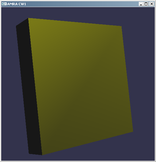
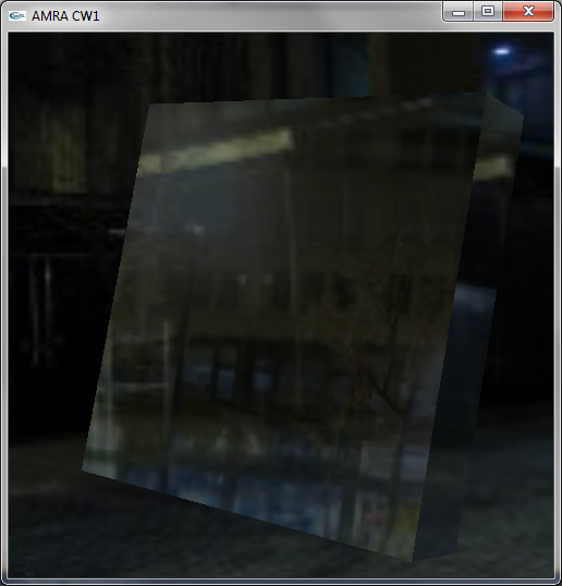
Compile and run the code. NOTE: Change the Working Directory to '../../..'. You can find this in Project -> Properties -> Configuration Properties -> Debugging (in the tree to the left). Once running, you should see an extruded square bathed in yellow light.
Read the instructions in the console window and interact with the application. Notice that when pressing 't', the model disappears. We would like 't' to switch between different models so that we may better observe lighting effects.
Find the display call in the code, and fill in the case/switch command so that the 't' key switches between the extruded square, a teapot, a sphere and a torus. Use the GLUT API with suitable parameters - it is already linked.
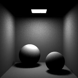
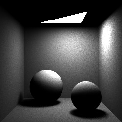
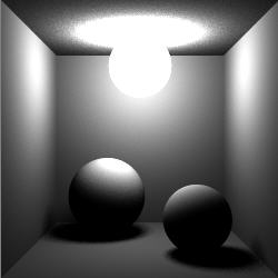
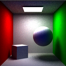
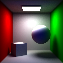
We would also like to add another light source to the scene, to observe more complicated lighting interaction. Find where the first light is setup in the code, and create another light of your choice to illuminate the model. You may need to refer to the OpenGL API documentation here. Once completed, you should have something that looks like this:
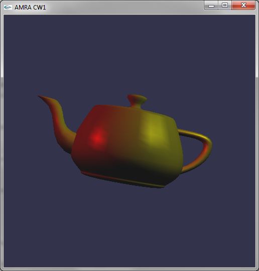
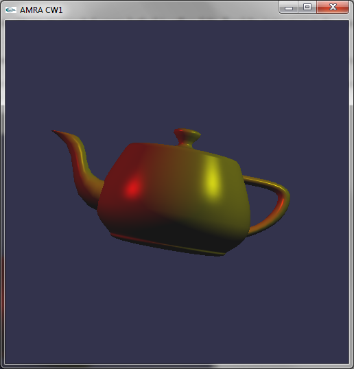
Pressing 's' will switch from using a per-vertex lighting shader (above left) to using a per-pixel lighting shader (above right). Notice the difference this causes by rotating the object with the mouse. Why are they different? Under which circumstances will these two different lighting techniques look the same? It may help to experiment with the parameters you use to create the objects.
Task 2:
We would now like to texture our object. Modify the per-vertex and per-pixel shaders to apply a texture to the object and light the object. Find the code that loads, links, and compiles the shader for the graphics card. Replicate this for your new shader. Note that any errors in your shader will be written to the console window for easier debugging.
ShaderGen is a tool from 3DLabs (now defunct) that converts fixed-function OpenGL into GLSL vertex and fragment shaders. It is included in the code package under the folder 'ShaderGen/bin'. Spend some time exploring ShaderGen to see how texturing can be added to objects and combined with lighting in shader code.
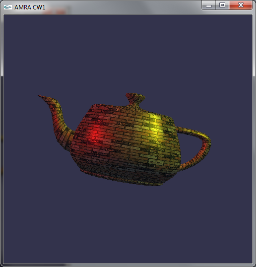
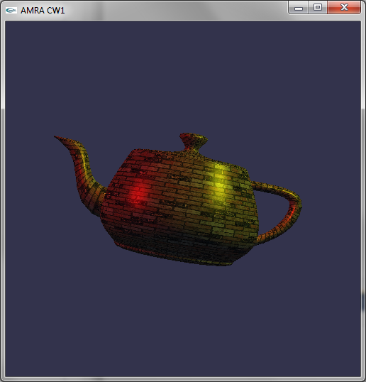
The function 'LoadDIBitmap' is provided to load 24bit RGB bitmap textures (like those included in the 'ShaderGen/textures' folder - note that some of these textures are RGB padded to 32bits - use the 'RGB' variants of the files if you do not see what you expect). Once loaded, use OpenGL calls to upload the texture to the graphics card, set any texture parameters correctly, and bind it for use. Note: Pay special attention to specular highlights!
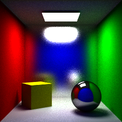
Once complete, your code should produce something like below. Why do these examples not look realistic?
Task 3:
We would now like to make our object very shiny, like chrome, so that it reflects the world around it. Currently, by changing material and light properties, we can generate a shiny highlight, but materials such as chrome are not accurately represented using these approaches. In COMP3080/GV10, coursework 1 showed how ray tracing could be used to generate such reflections of the world; however, this approach is expensive for real-time graphics. Instead, we will use environment mapping.
Environment mapping approximates the world outside the object using a texture. We use a specially formed texture, called a cube-map, which has six-sides. The texture is drawn as if we are inside the object, looking out at the world. Then, when we apply it to the object, it looks as if it is very shiny, reflecting the world around it.
A cube-map texture is provided in the folder 'cubemap'. You should start by drawing these textures to each side of a cube, and then drawing this cube around the object and the camera. This provides our outside world. Approach this part of the task by first correctly creating a GL_TEXTURE_CUBE_MAP texture out of the six-sided cube-map provided. 'draw.c' includes a function to draw a cube - make a new function using this example that now draws the cube textured with the cube-map.
Once that is complete, we now need to generate texture coordinates to make our cube map appear as if it is the reflection of the world. In Task 2, the texture is fixed to the object during rotation. With environment mapping for reflection, we want the texture to stay fixed while the object rotates - after all, the world is not rotating. Start by exploring ShaderGen's TEXTURE COORDINATE SET tab. This tab contains options for OpenGL's inbuilt texture coordinate generation. One of these is just what we're looking for - once you've found it, it may help to read up on texture coordinate generation. Integrate cube-map environment mapping into your shaders.
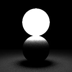
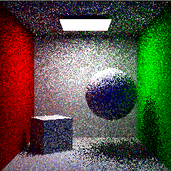
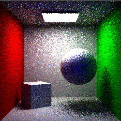
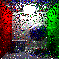
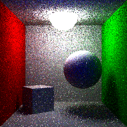
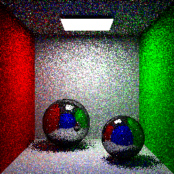
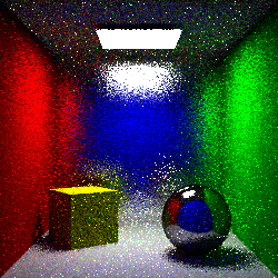
Once complete, your code should produce something like the following images:
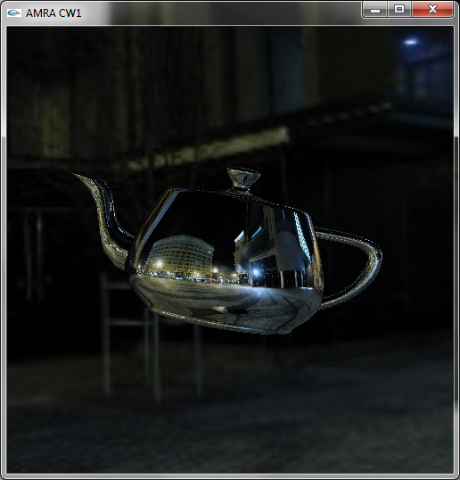
The left image still includes per-pixel lighting, but the scene does not look realistic. When using real-world sourced cube maps, why should we generally not use lighting with environment mapping?
Task 4:
We would now like to turn our object to glass. When light passes through a transparent material such as glass, some of the light is reflected and some of the light is refracted. The Fresnel equations describe this ratio, and Snell's Law defines the angle of the refracted ray. You will need to define a refractive index for your object. Air has a refractive index very close to 1, and most glasses have a refractive index around 1.5. Modify your shaders to implement refraction and make the object look like glass.
Importantly, here we are not concerned with physically accurate refraction. Given a ray incoming to the surface of our object, generate the refracted ray and assume it then goes off into the world and is not refracted again (as if the ray stays in glass until it reaches 'the world'). To be correct, we would again need to reflect/refract the ray when it exits the object, but you are not required to do this. We can produce something that looks convincing by performing just one refraction.
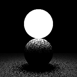
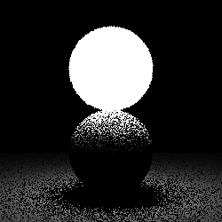
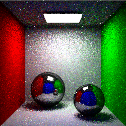
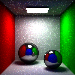
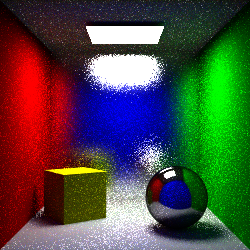
Once complete, your code should produce something like the following images:
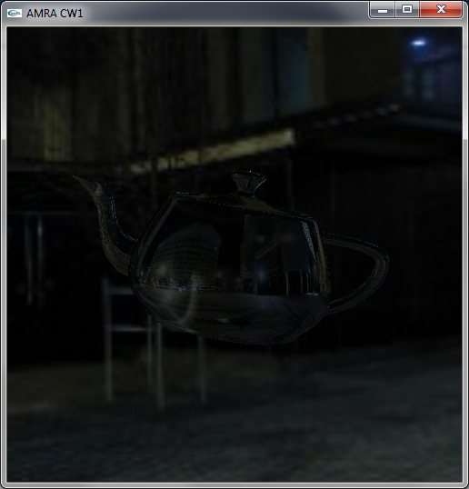
As this effect is only an approximation, which of the objects do you think produces the most convincing glass material? Which do you think produces the least convincing glass material? Why?
Task 5:
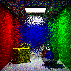
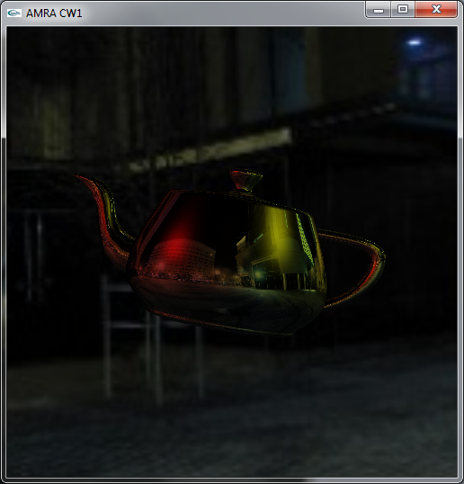
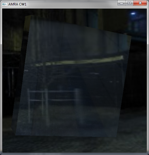
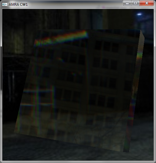
What if the refractive index of your object was not consistent? Have you ever peered through an old pane of glass and seen the world distort as you move your head? Implement 'bumpy' refraction to recreate this effect (left image). Use an appropriate example to show off this effect.
Different wavelengths of light are refracted by different amounts, producing dispersion (or chromatic aberrations - right image). How could this effect be implemented in a shader?
Looking at the Venus De Milo inspiration video in the references, we can see differences between the video and our result. What differences still remain, and how could these effects be achieved?
Write-up:
Please write a short report on your work, detailing how you solved each part of the coursework. Be sure to answer the questions that are in bold within this document. Include all relevant code along with screenshots to demonstrate your solution. Make sure that your report shows examples of all the required simulation effects - this may require side-by-side comparison shots with highlighting. Assignment on January 23rd. Submissions are due on Wednesday 6th February at 23:55. Electronic submission through Moodle. The report has to be in PDF format. Do not upload other document formats, such as Microsoft Word or Open Office.
References
OpenGL 2.1 Reference DocumentationGLSL Quick Reference Card
Venus De Milo inspiration!
Many cubemaps!
Arch cubemap courtesy of Paul Bourke.