The goal of this practical is to estimate the normals of a real object by processing its Reflectance Field, and then rerender it using a Blinn-Phong shading model.
You are given a set of images, captured by the Light Stage 6. Think of it as follows: the object is placed in the middle of a huge hemisphere where 253 lights are spread equally in all directions. We then take 253 photos of this object, using a different light each time. We know the orientation of each light, and our camera is calibrated so we know its position and orientation in world coordinates. We get a serie of photos, each one being illuminated differently, so we know what the objects looks like for every possible light orientation, and we can virtually relight the object exactly as we want by using a combination of those photos.
Here is the material you will need
- The dataset with 256x256 images (recommended if you want the algorithms to run fast), and the 256x256 mask.
- The dataset with 1024x1024 images, and the 1024x1204 mask.
- The matlab file that shows how to read the files one by one (you don't want to load them all in the same time).
- The light directions, and the camera matrix.
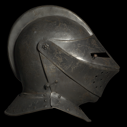
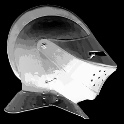
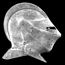
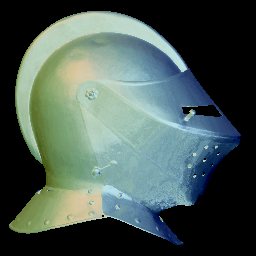
What we want to do today is first recover the normals of the object. You have to use the matte (mask) to only compute things that are on the object and not do anything for the background. Assuming that the object is mostly specular, and that we have photos of the object with every possible light direction, we know that every point will be shining light in at least one photo. For a given point, when the light is shining, how can we compute the normal? If we follow the Blinn-Phong model, then we can say that the shininesss is maximum when the half vector H is equal to the normal N of the surface. Therefore, if we calculate for each point what image gives the maximum intensity, it's easy to get an estimation of the normal by calculating the half vector. The first step then is to calculate a "map" that tells us for each point in which image we find the maximum intensity. We can also output the image of the object that we would have if it was lit in all direction: by keeping for each pixel the maximum intensity that we find accross all the images. To examplify, I display the map of lights that gives the maximum intensity at each pixel (black = light number 0, white = light number 253) and the "fully lit object":
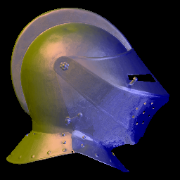
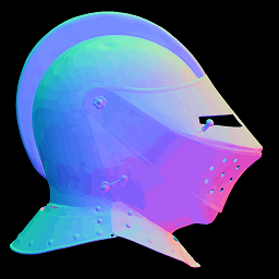
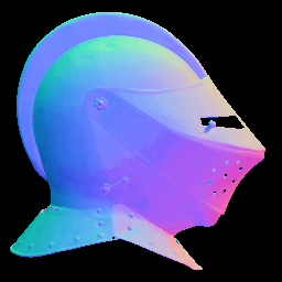
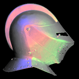
The next step is to estimate the normal map, given that we know the direction of each light, the extrinsic matrix of the camera (this goes from camera to world coordinates), and the orientation of the camera in camera space (it's the Z axis); don't forget to convert everything in Camera coordinate system (by taking the inverse matrix and transforming all the light directions; but be careful, we transform vectors and not points so we only want the first 3x3 components of the matrix). By mapping a normal (x,y,z) to a color (r,g,b) (I let you find the operation that does that), you should get a normal map that looks as follow:
The problem is that the set of lights that we get is still sparse, because we have only 253 different illuminations, so we won't get a very smooth normal map. One way to solve this problem is to use not one but multiple photos to estimate the normals. We can for example keep the 5 images that give the strongest intensities for each pixel, and interpolate them. For the moment, let's carry on with the simple normal map, and if you have time in the end you can try and implement that technique (instructions are given in the bottom of this page).
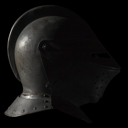
Now comes the fun part, we will actually rerender this object (remember, we don't have a 3D model, it is a real object!), by using the normal maps that we calculated. Using the Blinn-Phong model, we can use the camera direction, the normals, and the light direction (you decide where you want the light to be!), and calculate the color that the model returns for each pixel. The equation of the Blinn-Phong model is:
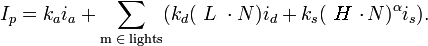
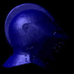
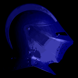
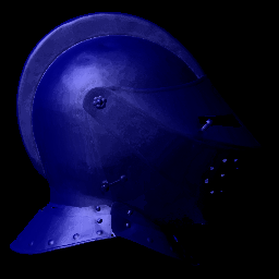
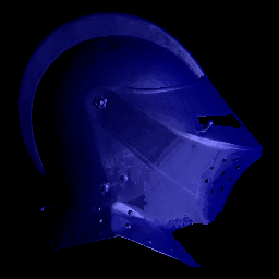
Where Ip is the final color at pixel p; Ka, Kd and Ks are the Ambient, Diffuse and Specular reflection constants; Ia is the ambient lighting; Id and Is are the Diffuse and Specular components of the light source; alpha is the shininess constant for the material, L is the direction of the light; N is the normal and H is the half vector, and is defined by H = (V+L)/2, where V is the view vector. For example, I chose a blue diffuse color, and a white specular color for my object, and I rerender it using Ka = 0, Ks = 0.5, Kd = 0.5, alpha = 20, for a light being first on the left, and then on the right of my object. I obtain those images:
You are invited to play with the settings, set different colors, different intensities, different light sources, and even multiple light sources.
Now we can get into the interpolation process to get smoother normals. In order to get rid of the quantisation due to discrete lighting directions, a weighted sum of the lighting directions of the top-k brightest reflections can be used. To this end we recommend using Unstructured Lumigraph (ULR) interpolation. ULR interpolation was originally intended to blend between k-1 or a set of k closest camera views, but it can also be seen as a method for general scattered data interpolation.
We propose using a simplified reformulation of the original ULR that uses relative weights r_i (<1), which in this case would be reflection intensities. Without loss of generality, let r_k be the k-th largest r_i. The algorithm first determines intermediate weights:
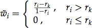
Note how the k-th largest relative weight is mapped to a w_i of zero. (This will lead to the darkest reflection's lighting direction to ease in and out smoothly across the surface.) Normalization yields the final weights:

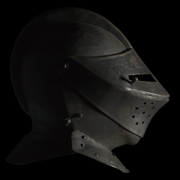
A key property of ULR interpolation is that for smoothly changing input weights r_i, the resulting weight vector changes smoothly as well. In the case of lighting directions to be blended across a surface, this particularly means that the influence of individual directions blends in and out smoothly, as long as there are no discontinuities in the variation of r_i. Now you can try to redo the normal estimation using that technique (and take for example k = 5 or 10). You should get smoother results:
Again, play with the light and colours settings to get nice outputs:
The last image was generated using white material and three coloured lights. Something to try (probably at home) is to render the helmet without calculating the normals, but by using three images from the data where the lights are oriented in similar directions to the desired virtual lights, blend/scale those three images (for example to simulate a red light you can only take the red channel of one image) and compare it with the Blinn-Phong render.
Now think about the following: how would you estimate the normals if the object was not specular, but Lambertian? Using the photos, how would you display the diffuse color of the object, without displaying any reflection?
Finally, if you think that you can generate any particularly artistic / crazy images, send us an email: we're happy to exhibit them on this page.