GV12/3072
Coursework 4
This coursework is on
color imaging and color constancy. For a good pass in the coursework
(60%), you need to do the core section. To get full marks (100%) you
must do ALL the additional sections. I recommend you use matlab.
Hand in a short report on your work, which should be two written sides
of A4 at most, plus any pictures and plots showing your results and a
print out of your code. Write a short description of the methods you
used for each part together with any conclusions you have drawn from
your experiments. Make sure it is clear what commands you used to
generate each of the pictures you include. Print the images in color
for the deadline!
The hand-in deadline for this coursework is 12:00 noon on 15th
December.
Hand
your report into the CS departmental office. Make sure you attach a
completed coursework
cover sheet to your work.
Core section
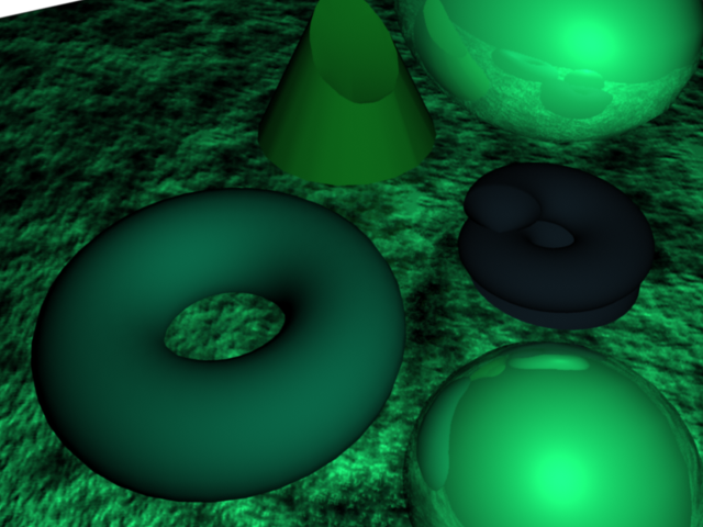
Here is an image of
three colored objects (helix, truncated cone, and torus), with two
decorative mirror-spheres (to be ignored below):
In general, we seek color image descriptions that characterize the
different objects' materials in a way that is independent of a) the
geometry of the illuminated surface
(slides, p.~28), b) the illumination color
(p.~52), or sometimes c) both. In this case:
- Define regions*
corresponding to each of the three objects in the image above. Show the
mask or outline of the regions. Generate
plots that show the occupancy of the RGB cube (i.e. which colors appear
in the object's image region) for each object. A nice way to do this is
to plot each object using a different color. Look up the matlab
function
plot3 and see a sample here
to see
how to generate a simple occupancy plot. Comment on how the color
distributions vary among objects.
- Compute the mean and covariance of the color distribution for
each object under this illumination (so you are modeling each object's
colors as a normal distribution, i.e. Gaussian). Then, construct a table of
separations
between the three objects' color distributions. The
measure of distance D between
two Gaussian distributions with means m1 and m2
and covariances C1 and C2 is
D:=(1/8)(m1-m2)T C-1 (m1-m2) + (1/2) ln[ det(C) / sqrt(det(C1) * det(C2) ) ],
known as the Bhattacharyya distance. Here, C
is the per-element average of the two constituent covariance matrices,
and note that you may find Matlab's pinv() function useful to take the
pseudoinverse instead of the inverse. Comment (only) on how
reliably you expect a computer vision system, that uses the unprocessed
color information alone, to recognize and distinguish between these
different object surfaces in unknown illumination. Note: the product of
determinants may come out negative, so you may need to take abs() of it.
- Construct occupancy plots after correction for
surface geometry, i.e. in "normalized color" space.
Show the image in this new color space. Recompute the mean and
covariance-matrices in the normalized color space. Recompute the table
of separations between each pair of distributions and comment on
whether you would expect any improvement in object surface recognition
using normalized color. Note: normalization involves division, so
consider a reasonable solution for when the denominator is zero.
- Construct occupancy
plots for the image above after correction for illumination color only. Show the image in this
new color space.
Additional section
To get more than a
basic pass, do this:
(Note, unlike the previous courseworks, these 40% of the marks should
require less effort than usual)
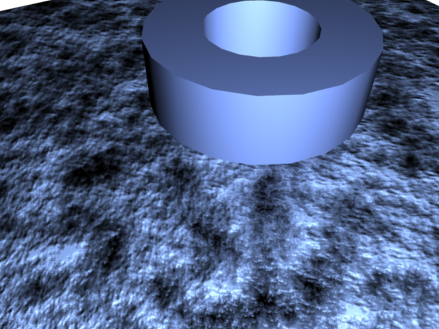
- Correct the below image
for illuminated surface geometry.
- Correct the below image
for illumination color.
- What color (red, green
or blue) is the pipe-shape in this second image? It
may seem bright gray, but
actually has some saturation. Correct for anything else you need, and
show your work, justifying your answer. There are several acceptable
solutions & explanations.
*= You can use imfreehand(), for example:
imshow(I);
h = imfreehand
IbwMask = createMask(h);