From Camino

Tutorials: QBallTutorial

Tutorial: Q-Ball Imaging

This tutorial illustrates how to use Q-Ball imaging [1] to reconstruct multiple fibre directions in single voxels. Q-Ball is a linear reconstruction method capable of resolving complex sub-voxel structure and, in particlular, capable of resolving multiple fibre directions in a single voxel. In contrast to the PAS method used in the pig brain tutorial, Q-Ball is a linear reconstruction method and as such is computationally less demanding, although it is generally less sensitive to crossing fibres.

This tutorial demonstrates Camino command pipelines that generate images of Q_Ball orientation distribution functions (ODF) and generate statistics from them.

Data & Scheme File

The data used in this study is the same as that used in the pig brain tutorial. The pig brain tutorial discusses the necessary steps to preprocess data into voxel order, as expected by Camino. If your data is in Analyze format, the program analyze2voxel will convert the data into voxel order. The command

analyze2voxel pigBrain > pigBrain.Bfloat

will convert the analyze files pigBrain.hdr, pigBrain.img to big endian voxel order format.

Scan parameters and gradient directions are contained in the camino schemefile for the dataset. Schemefiles for the pig brain dataset are also available in the pig brain tutorial.

Generating a Q-Ball ODF map

This section shows how to use Camino to create a spherical radial basis function (sRBF) representation of Q-Ball ODFs in each voxel of a brain volume. (This is Tuch's original approach in [1]; later we will look at spherical harmonic Q-Ball, which is more economical.) We will then visualize the ODFs of one slice of brain data using sfplot.

Prior to calculating the Q-Ball ODFs, we will perform a diffusion tensor reconstruction of the data. There are two reasons for doing this. First, we use the DT fit to test that none of the directions are flipped using the commands:

dtfit pigBrain.Bfloat pigBrain.scheme > pigBrainDTs.Bdouble
dteig < pigBrainDTs.Bdouble > pigBrainDT_EIGs.Bdouble
pdview -inputmodel dteig -datadims 128 128 10 < pigBrainDT_EIGs.Bdouble

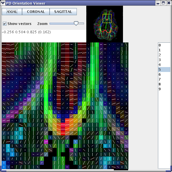
Figure 1a principal eigenvectors from a diffusion tensor reconstruction generated after the schemefile has been corrected

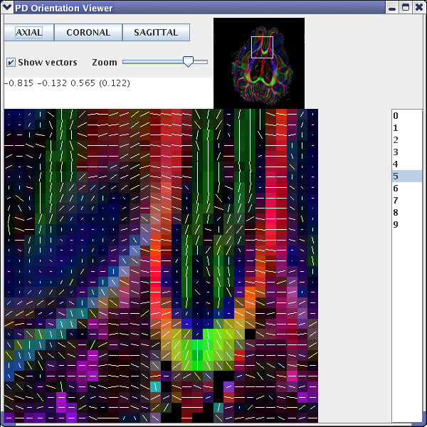
Figure 1b - principal eigenvectors from a diffusion tensor reconstruction when an incorrect schemefile is used

If we examine an axial slice in the centre of the brain volume, we should see that the principal directions of the diffusion tensor follow the white-matter tracts (see fig 1a). However, if one of the directions is flipped, for example the y direction, then we will see an image similar to that of fig 1b. We also use the diffusion tensor reconstruction to create the FA map for the background image. This is achieved using the fa program

fa < pigBrainDTs.Bdouble > pigBrainDT_FA.img

The first stage required for Q-Ball reconstruction is the generation of the Q-Ball reconstruction matrix. This matrix transforms the data from a sphere in q-space to the ODF. To calculate the Q-Ball reconstruction matrix we use qballmx:

qballmx -schemefile pigBrain.scheme > qballMatrix.Bdouble

This command uses sensible defaults for the various parameters of the Q-Ball algorithm and is equivalent to

qballmx -schemefile pigBrain.scheme -basistype rbf -rbfpointset 246 -rbfsigma 0.2618 -smoothingsigma 0.1309 > qballMatrix.Bdouble

The extra options can be changed to adapt the behaviour of the algorithm, see [1,2] for details. If the program has run successfully, you will see information about the basis functions used as well as their settings on the command console. Record this information for future reference as you will need it later.

We can check that the settings (i.e. the number ODF basis functions and their widths) give reasonable results by generating some test ODFs using synthetic data from datasynth using the commands

datasynth -testfunc 3 -schemefile pigBrain.scheme -snr 16 -voxels 10 > testData.Bfloat
linrecon testData.Bfloat pigScheme qballMatrix.Bdouble -normalize > testODF.Bdouble

To visualize this test data, we can create a basic greyscale image using sfplot:

sfplot -inputmodel rbf -rbfpointset 246 -rbfsigma 0.2618 -xsize 1 -ysize 10 -minifigsize 60 60 -minifigseparation 1 1 -minmaxnorm < testODF.Bdouble > testODF.gray

Figure 2 - image of ODFs from synthetic data generated using sfplot

To view the image on a UNIX machine with Image Magick installed, use the command display -size 610x61 testODF.gray (some versions of ImageMagick may require the flag -depth 8 in addition to the -size 610x61 flag). The file extension directly affects how display reads the file. For those that are not using UNIX, the file can be loaded into matlab using the following command:

fid = fopen('testODF.gray','r','b');
data=fread(fid,'char');
fclose(fid);
image=uint8(reshape(data,610,61));
imshow(image,[]);

Once you have found settings that give reasonable results, you calculate the ODFs for each voxel of the pig brain dataset using:

linrecon pigBrain.Bfloat pigBrain.scheme qballMatrix.Bdouble -normalize -bgthresh 200 > pigBrainODF.Bdouble

We choose the value for -bgthresh by thresholding the b0 image such that the background is masked while brain voxels remain. Use any image viewer (MRIcro/ITKsnap/Matlab) to compare foreground and background intensities in the b0 image and pick a value that lies between the two.

To create a colour-coded image using sfplot, you first need to split the data into slices. For details on how to do this, please refer to the pig brain tutorial. Here, we will use the UNIX split command

split -b $((128*128*248*8)) pigBrainODFs.Bdouble splitBrain/pigBrainODFs_slice
split -b $((128*128*8)) pigBrainFA.img splitBrain/pigBrainFA_slice

To create a colour-coded image, we add the flag -dircolcode. The sfplot command in full is

sfplot -inputmodel rbf -rbfpointset 246 -rbfsigma 0.2618 -xsize 128 -ysize 128 -minifigsize 30 30 -minifigseparation 2 2 -minmaxnorm -dircolcode -backdrop splitBrain/pigBrainFA_sliceaa < splitBrain/pigBrainODFs_sliceaa > pigBrainODFs_sliceaa.rgb

This image can be viewed in display using the same command as before, i.e display -size 4096x4096 pigBrainODFs_sliceaa.rgb. In Matlab, use the commands

fid = fopen('pigBrainODFs_sliceaa.rgb','r','b');
data=fread(fid,'unsigned char');% image in format [r_1, g_1, b_1, ..., r_N, g_N, b_N]
fclose(fid);
image=reshape(data,3, 4096, 4096);
image=uint8(permute(image, [2 3 1]));\\ % need the matrix to be in the format [x, y, rgb channel]
imshow(image,[]);

Figure 3 - image of ODFs from pig brain dataset generated using sfplot

Using sfpeaks to get useful information from Q-Ball ODFs

Camino also implements the spherical harmonic (SH) Q-Ball reconstructions of Descoteaux [3] and Mukherjee [4]. We will now create an SH representation of the Q-Ball ODFs and use sfpeaks to find the peaks of the ODF in each voxel, which we will view in pdview. sfpeaks is a program that finds a wide range of features for any multiple-fibre reconstruction (such as PASMRI, Q-Ball, Spherical Deconvolution). In particular, for any given voxel it outputs the number of peaks found, the mean of the function, the orientations and strengths of the peaks as well as the Hessian (or matrix of second partial-derivatives, which describes the curvature of the peak) of each peak. This information is used in several Camino programs, inluding the tractography and statistics programs. To create a spherical harmonic representation of the ODF, you will need to calculate a new Q-Ball matrix with the flag -basistype sh and then run linrecon. The full commands are

qballmx -schemefile pigBrain.scheme -basistype sh -order 4 > qballMatrix_SH4.Bdouble
linrecon pigBrain.Bfloat pigBrain.scheme qballMatrix_SH4.Bdouble -normalize -bgthresh 200 > pigBrainODFs_SH4.Bdouble

The command to run sfpeaks is

sfpeaks -inputmodel sh -order 4 -numpds 3 < pigBrainODFs_SH4.Bdouble > pigBrainODFs_SH4_PDs.Bdouble

In addition to displaying the principal eigenvectors of the diffusion tensor, pdview also allows you to view the output of sfpeaks. To do this, use the flag -inputmodel pds. The background map uses the trace of the Hessian (i.e. the sharpness) of the dominant peak of each ODF. Alternatively, you can specify another greyscale background map (for example, a fractional anisotropy image) using the flag -scalarfile [filename]. The color-coding is added automatically by pdview. The command is

pdview -inputmodel pds -numpds 3 -datadims 128 128 10 < pigBrainODFs_SH4_PDs.Bdouble

Here is an image of a pdview output. Note that only the 2 largest peaks are displayed.

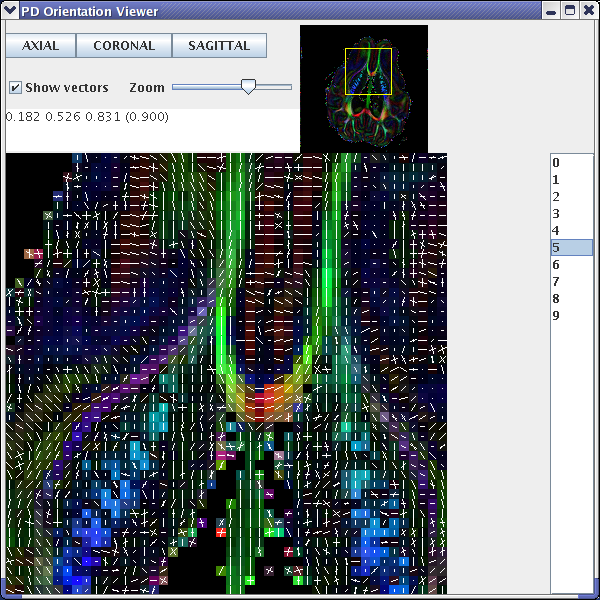
Figure 4 - Using pdview to show the fibre-orientation estimates in each voxel of a SH Q-Ball reconstruction. The background map is generated using the trace of the Hessian, which describes peak sharpness, of the principal peak of each Q-Ball ODF.

References

[1] D. S. Tuch. Q-Ball Imaging, Magnetic Resonance in Medicine, 52:1358-1372, 2004.
[2] D. C. Alexander. Multiple fibre reconstruction algorithms for diffusion MRI, Annals of the New York Academy of Sciences 1046:113-133 2005.
[3] M. Descoteaux. A fast and robust ODF estimation algorithm in Q-Ball imaging, Biomedical Imaging: Macro to Nano. 3rd IEEE International Symposium, 81-84, 2006
[4] C.R. Hess et al. Q-ball reconstruction of multimodal fiber orientations using the spherical harmonic, Journal Magnetic Resonance Imaging, 56:104-117, 2006.