From Camino

Tutorials: Tutorial: detecting crossing fibres

This tutorial uses Camino to generate fractional-anisotropy, colour-coded direction and voxel-classification maps. The voxel classification maps indicate which voxels exhibit isotropic diffusion, anisotropic Gaussian diffusion (adequately modelled by a single diffusion tensor) and non-Gaussian displacements (the diffusion tensor model fails), which are likely fibre crossings.

Data

The data set in this case study comes from a post-mortem porcine brain and was kindly provided by Tim Dyrby from The Danish Research Centre for Magnetic Resonance, Copenhagen University Hospital, Hvidovre, Denmark. The data set is intended for demonstration and testing of the Camino software package only. If you wish to use this data for other purposes, such as publications, other web sites or commercial enterprises, please contact Tim at (timd|at|drcmr.dk) before doing so. You can download the data set . The acquisition uses a spherical acquisition scheme with 61 unique gradient directions. The gradient directions come from the file camino/PointSets/Elec061.txt and minimize the electrostatic energy for 61 pairs of equal-and-opposite point electrical charges free to move on the surface of the sphere. The procedure outlined in [Jansons and Alexander, Inverse Problems, Vol 19, pp 1031-1046, 2003] computed them. The diffusion-weighting gradient strength G = 61 mT m^-1; pulse onset separation DELTA = 30ms; pulse width delta = 23ms; TE = 60ms; b = 3146 s mm^-2; NEX=2. The protocol also includes 3 acquisitions with no diffusion weighting. The image has 10 slices with in-plane resolution 128x128; voxel size 0.5x0.5x0.5 mm³. You can download the data here.

Scheme File

Before we can process the data, we must create a scheme file that tells Camino about the acquisition sequence. The scheme file is a text file; the Camino man page (camino/man/man1/camino.1) specifies the available formats. The pointset2scheme program converts point sets to scheme files. The point set for this data is stored in pigPoints.txt. The appropriate scheme file format depends on the application and the available information about the image acquisition. In this case, we know most of the imaging parameters, so we'll generate a detailed scheme file:

The "version" argument tells the program that we want to describe a Stejskal-Tanner sequence, which uses two rectangular gradient pulses of equal duration. The "dwparams" argument is followed by the parameters of the sequence: gradient strength (0.061 T / m), pulse separation (0.03 s), pulse duration (0.023 s), and echo time (0.06 s). Alternatively, we could compute the b-value for the scheme, 3146 s/mm^2, and created a less detailed scheme file:

For most applications, different scheme files are equivalent as long as they describe the same b-value. Some programs, like the monte-carlo diffusion simulation, require a more detailed description of the pulse sequence.

Fit the diffusion tensor

Each acquisition from the scanner is in an analyze format file NEX2_s_20060127_001_semsdw_15_image??, where ?? goes from 01 to 64; 01-03 are the b=0 images and 04-64 are the diffusion-weighted images with gradients in the same order as the scheme file.

To fit the diffusion tensor in each voxel we can use analyzedti:

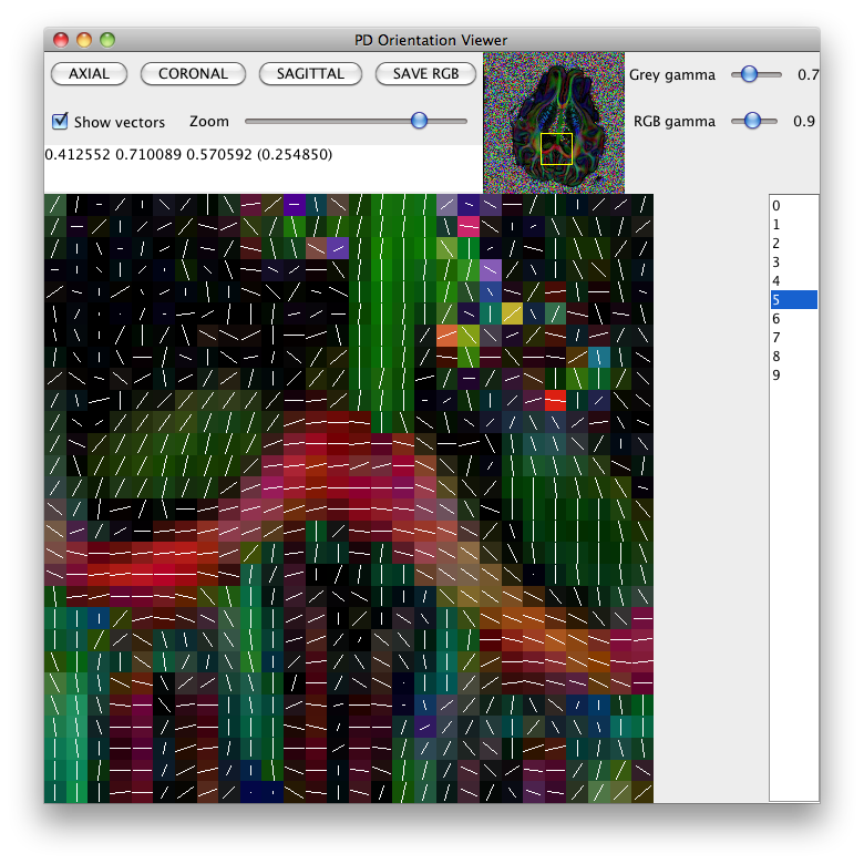
This command produces several Analyze images, and some Camino raw data files. All output is prepended with pig_. See the man page for analyzedti for more details. We can check the reconstruction using pdview:

Diffusion tensor plot

The command sfplot creates plots of diffusion MRI reconstructions over slices. In particular, it can create plots of the diffusion tensor over a slice. It can also create plots of other reconstructed features, such as the PAS or q-ball ODF; see for example the Parallel PASMRI case study or the sfplot man page. The following commands create a plot of the DT over slice 5 of the pig brain data set. We start by creating a fractional anisotropy map to use as background for the plot:

fa < pig_dt.Bdouble | shredder $((128*128*8*4)) $((128*128*8)) $((128*128*8*10)) > PigBrainFA_SLICE05.Bdouble

The command above uses shredder to pick out the fifth slice of the FA map over the whole volume; each slice contains 128*128*8 bytes, as the FA in each of the 128*128 voxels per slice is an 8-byte double. Now create the plot itself:

shredder $((128*128*8*8*4)) $((128*128*8*8)) $((128*128*8*8*10)) < pig_dt.Bdouble | sfplot -xsize 128 -ysize 128 -inputmodel dt -backdrop PigBrainFA_SLICE05.Bdouble -dircolcode -maxd 0.4E-9 -projection 2 1 > PigBrain05_PAS.rgb

The man page for sfplot explains the options in detail. Briefly, the first two (-xsize 128 -ysize 128) define the size of the image array; -inputmodel dt says that the program is reading in diffusion tensor data; -backdrop PigBrainFA_SLICE05.Bdouble says to use the FA map we just created as the background; -dircolcode defines the colour scheme to use and encodes directions as colours so that left-right oriented tensors are predominantly red, anterior-posterior green and superior inferior blue (other schemes are available); -maxd 0.4E-9 specifies the scale of the tensors, as the default is larger as it was chosen for in-vivo imaging; -projection 2 1 specifies the orientations of the DTs with respect to the image. In practice, you need to experiment with some of these settings to get good images for particular acquisitions. The shredder command above picks out the fifth slice of the diffusion tensor data set.

The command outputs a figure in raw rgb format. You can convert it to something more convenient using, for example, ImageMagick's convert command:

convert -size 2048x2048 -depth 8 PigBrain05_PAS.rgb PigBrain05_PAS.png

Here is the figure output (click to see the full size image):


To make the figure look a bit nicer, I've used a version of the PigBrainDT.Bdouble file with the background threshold set to 500.

Voxel Classification

The command voxelclassify classifies each voxel as isotropic, anisotropic Gaussian or non-Gaussian using the algorithm in [Alexander, Barker and Arridge, MRM, Vol 48, pp 331-340, 2002]. In isotropic and anisotropic Gaussian voxels, the diffusion tensor model works well. Non-Gaussian voxels are likely fibre crossings where the diffusion tensor fails. The algorithm requires you to select thresholds for separating the three classes. First run:

voxelclassify -inputfile PigBrain.Bfloat -bgthresh 500 -schemefile PigBrain.scheme -order 4 > PigBrainVC.Bdouble

To choose thresholds, run the vcthreshselect program giving it the output of the command above:

vcthreshselect -inputfile PigBrainVC.Bdouble -datadims 128 128 10 -order 4

A window appears that looks like this: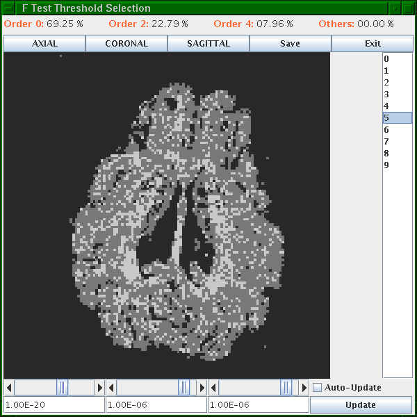


Black voxels are isotropic ("Order 0") or background, dark gray are anisotropic Gaussian ("Order 2") and light gray are non-Gaussian ("Order 4"). The light gray ones are likely fibre crossings. Scroll through the slices using the list on the right. Set the thresholds using the scroll bars or text fields at the bottom. At good threshold settings, the order 4 voxels should be fairly clustered, ie as few isolated order 4 voxels as possible with still a reasonable fraction of order 4 voxels overall. Around 5 to 10 percent order 4 voxels is typically about right.

Once you have chosen thresholds, make a note of them and generate the classified volume using voxelclassify with specified thresholds:
voxelclassify -inputfile PigBrain.Bfloat -bgthresh 500 -schemefile PigBrain.scheme -order 4 -ftest 1.0E-20 1.0E-7 1.0E-7 > PigBrainVC.Bint

The output of this command has type int and every voxel contains either -1 for background or 0, 2 or 4 indicating the classification order. A nice visualization of the results highlights the fibre crossings on the fractional anisotropy map. This is simple in Matlab:

>> fid = fopen('PigBrainVC.Bint', 'r', 'b');
>> vc=fread(fid, 'int');
>> fclose(fid);
>> vc=reshape(vc, 128,128,10);
>> % Repeat for FA
>> fid = fopen('PigBrainFA.Bdouble', 'r', 'b');
>> data = fread(fid, 'double');
>> fclose(fid);
>> fa = (reshape(data, 128,128,10) - min(data))/(max(data) - min(data));
>> for i=1:10
>> im(:,:,1) = fa(:,:,i).*(1-0.5*(vc(:,:,i)>=4)) + 0.5*(vc(:,:,i)>=4);
>> im(:,:,2) = fa(:,:,i).*(1-0.5*(vc(:,:,i)>=4)) + 0.5*(vc(:,:,i)>=4);
>> im(:,:,3) = fa(:,:,i);
>> imwrite(im, sprintf('/tmp/favc%02i.png', i));
>> end
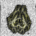
Here is the image for slice 5: